Compare two columns row by row

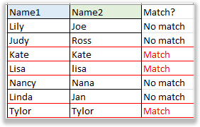
Below is a dataset (the range B2:C8) where I need to check if the names in column B are the same as those in column C within the same row.

This part provides two examples for explaining how to compare two columns row by row

• Example 1: Compare cells in the same row
• Example 2: Compare cells in the same row in case sensitive

Example 1: Compare cells in the same row

Generally, if you want to compare two columns row by row for exactly matching, you can use below formula:

=B2=C2

Press Enter key and drag fill handle down to cell D8. If the formula returns TRUE, the values in the same row of two columns are totally same; if it returns FALSE, the values are different.

Or you can display specific texts for showing matches or mismatches by using IF function like this:

=IF(B2=C2,"Match","No match")

The result may look like below:

Example 2: Compare cells in the same row in case sensitive

If you want to compare two columns row by row for case sensitive, you can use the formula combined IF and EXACT functions.

IF(EXACT(B2,C2), "Match", "Mismatch")

Press Enter key to get the first result, then drag auto fill handle to cell D8.

In above formula, you can change the texts “Match” and “Mismatch” to your own description.

Compare multiple columns in the same row

Sometimes, you may want to compare more than two columns in the same row, such as the data set (the range B2:D7) as below screenshot shown. In this section, it lists different methods on comparing multiple columns.

Here, it is split into two parts to provide detailed instructions on comparing multiple columns in the same row.

• Example 1: Compare multiple columns and find matches in all cells in the same row
• Example 2: Compare multiple columns and find matched in any two cells in the same row

Example1: Compare multiple columns and find matches in all cells in the same row

To find full matches across columns in the same row, the below formula can help you.

=IF(COUNTIF($B2:$D2, $B2)=3, "Full match", "Not")

Press Enter key to get the first comparing result, then drag auto fill handle over to cell E7.

Example 2: Compare multiple columns and find matched in any two cells in the same row

Sometimes, you want to find out if any two columns in the same row are matched, you can use below IF formula.

=IF(COUNTIF($B2:$D2,$B2)>=2,"Match","No match")

Press Enter key, and drag fill handle over to cell E7.

Compare two or multiple columns row by row and highlight matches or differences

If you want to compare two columns or more columns and highlight the matches or differences, this section will introduce two methods on handling these jobs.

There are two examples for comparing and highlighting matches and differences

• Example 1: Compare two columns and highlight full matches in all cells in the same row or any two cells in the same row
• Example 2: Compare two columns and highlight differences in the same row

Example 1: Compare two columns and highlight full matches in all cells in the same row or any two cells in the same row

For highlighting matches in all cells or any two cells in the same row, the Conditional Formatting feature can help you.

1. Select the range that you use, then click Home > Conditional Formatting > New Rule.

2. In the New Formatting Rule dialog

1. Choose Use a formula to determine which cells to format from the Select a Rule Type section
2. Use below formula in the Format values where this formula is true textbox.
   

   =COUNTIF($B2:$D2, $B2)=3

3. Click Format.

3. In the Format Cells dialog, then choose one fill color or other cell formatting to outstand the rows. Click OK > OK to close dialogs.

Now only rows within which all cells are matching will be highlighted.

Example 2: Compare two columns and highlight differences in the same row

If you want to highlight the differences in the same row, which means it compares column cells one by one, and find the different cells according to the first column, you can use Excel built-in feature-Go To Special.

1. Select the range that you want to highlight row differences, and click Home > Find & Select > Go To Special.

2. In the popping Go To Special dialog, choose Row differences option. Click OK.

Now the row differences have been selected.

3 Now keep the cells selected, click Home > Fill Color to select one color from the drop-down menu.

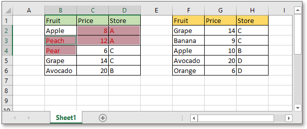
Compare two columns in cells for unique and duplicate data

In this part, the data set (the range B2:C8) is shown as below, and you want to find all values which are in both column B and column C simultaneously, or, find the values only in column B.

This section lists 4 different methods for comparing two columns in cells, and you can choose one of the following based on your needs.

• Example 1: Compare two columns in cells and display comparing result in another column
• Example 2: Compare two columns in cells and select or highlight duplicate or unique data with a handy tool
• Example 3: Compare two columns in cells and highlight duplicate or unique data
• Example 4: Compare two columns in cells and list exact duplicates in another column

Example 1: Compare two columns in cells and display comparing result in another column

Here you can use the formula which is combined with IF and COUNTIF function to compare two columns and find the values that are in column B but not present in column C.

=IF(COUNTIF($C$2:$C$8, $B2)=0, "No in C", "Yes in C")

Press Enter key and drag autofill handle over to cell D8.

Example 2: Compare two columns in cells and select or highlight duplicate or unique data with a handy tool

Sometimes, after comparing two columns, you may take other actions on the matches or difference, such as selection, deletion, copy and so on. In this case, a handy tool – Select Same & Different Cells of Kutools for Excel can directly select the matches or difference for better doing next operation, also can directly highlight the values.

After free installing Kutools for Excel, click Kutools > Select > Select Same & Different Cells. Then in the Select Same & Different Cells dialog, please do as below:

1. In the Find values in and According to sections, choose two columns separetedly that used to compare with.
2. Choose Each row option.
3. Choose Same values or Different Values as you need.
4. Specify whether color the selected values and click OK.

A dialog pops out to remind you the number of values that have been found, click OK to close the dialog. And at the same time, the values have been selected, now you can delete or copy or do other operations.

If you tick the Fill backcolor and Fill font color checkboxes, the result is shown as this:

Example 3: Compare two columns in cells and highlight duplicate or unique data

The Conditional Formatting feature in Excel is powerful, here you can use it to compare two columns in cells and then highlight the differences or matches as you need.

1. Select two columns that you will compare with, then click Home > Conditional Formatting > Highlight Cells Rules > Duplicate Values.

2. In the popping Duplicate Values dialog, choose a highlighting format you need from the drop-down list of values with.

3. Click OK. Then the duplicates in two columns have been highlighted.

Example 4: Compare two columns in cells and list exact duplicates in another column

If you want to list the matching values in another column after comparing two columns cell by cell in case sensitive, here the below macro code can help you.

1. Enable the sheet that you want to compare two columns, then press Alt + F11 keys to display the Microsoft Visual Basic for Applications window.

2. Click Insert > Module in the Microsoft Visual Basic for Applications window.

3. Then copy and paste below code to the new blank module script.

VBA: List duplicates in beside column after comparing two columns

Sub ExtendOffice_FindMatches()
'UpdatebyKutools
Dim xRg, xRgC1, xRgC2, xRgF1, xRgF2 As Range
Dim xIntSR, xIntER, xIntSC, xIntEC As Integer
On Error Resume Next
SRg:
Set xRgC1 = Application.InputBox("Select first column:", "Kutools for Excel", , , , , , 8)
If xRgC1 Is Nothing Then Exit Sub
If xRgC1.Columns.Count <> 1 Then
    MsgBox "Please select single column"
    GoTo SRg
End If
SsRg:
Set xRgC2 = Application.InputBox("Select the second column:", "Kutools for Excel", , , , , , 8)
If xRgC2 Is Nothing Then Exit Sub
If xRgC2.Columns.Count <> 1 Then
    MsgBox "Please select single column"
    GoTo SsRg
End If
Set xWs = xRg.Worksheet
For Each xRgF1 In xRgC1
    For Each xRgF2 In xRgC2
        If xRgF1.Value = xRgF2.Value Then xRgF2.Offset(0, 1) = xRgF1.Value
    Next xRgF2
Next xRgF1
End Sub

4. Press F5 key to run the code, there are two dialogs popping out one by one for you to select two columns separately. Then click OK > OK.

The matches have been automatically listed in the right column of the two columns.

Compare two lists and pull matching data

Here we introduce two different scenarios for comparing two lists and pulling data.

• Example 1: Compare two columns and pull the exact matching data
• Example 2: Compare two columns and pull the partial matching data

Example 1: Compare two columns and pull the exact matching data

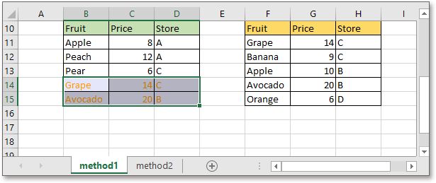
For example, there are two tables, now you want to compare column B and column E, then find the relative prices from the column C and return them in column F.

Here it introduces some helpful formulas to solve this job.

In the cell F2 (the cell you want to place the returned value in), use one of below formulas:

=VLOOKUP(E2,$B$2:$C$8,2,0)

Or

=INDEX($B$2:$C$8,MATCH(E2,$B$2:$B$8,0),2)

Press Enter key, and the first value has been found. Then drag auto fill handle down to cell F6, all values have been extracted.

Example 2: Compare two columns and pull the partial matching data

If there are some minor differences between the two compared columns as below screenshot shown, the above methods cannot work.

In the cell F2 (the cell you want to place the returned value in), use one of below formulas:

=VLOOKUP("*"&E2&"*",$B$2:$C$8,2,0)

Or

=INDEX($B$2:$C$8,MATCH("*"&E2&"*",$B$2:$B$8,0),2)

Press Enter key, and the first value has been found. Then drag auto fill handle down to cell F6, all values have been extracted.

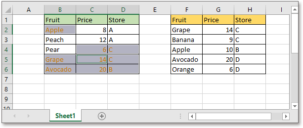
Compare two columns and find missing data points

Supposing there are two columns, column B is longer, and column C is shorter as below screenshot shown. Compared with column B, how to find out the missing data in column C?

• Example 1: Compare two columns and find the missing data points
• Example 2: Find the missing data points and list them in another column (using a handy tool)
• Example 3: Compare two columns and list missing data in below

Example 1: Compare two columns and find the missing data points

If you only want to identify which data is missing after comparing two columns, you can use one of below formulas:

=ISERROR(VLOOKUP(B2,$C$2:$C$10,1,0))

Or

=NOT(ISNUMBER(MATCH(B2,$C$2:$C$10,0)))

Press Enter key, then drag auto fill handle over cell D10. Now if the data is in both column B and column C, the formula returns FALSE, if the data is only in column B but misses in column C, the formula returns TRUE.

Example 2: Find the missing data points and list them in another column (using a handy tool)

If you want to do some follow-up operation on the missing data after comparing two columns, such as listing the missing data in another column or supplementing the missing data below the shorter column, you can try a handy tool-Select Same & Different Cells of Kutools for Excel.

After installing Kutools for Excel, click Kutools > Select > Select Same & Different Cells. Then in the Select Same & Different Cells dialog, do as below:

1. In the Find values section, choose the longer column that contains the complete list.
2. In the According to section, choose the shorter column which misses some data.
3. Choose Each row option.
4. Choose Different Values option. Click OK.

A dialog pops out to remind you the number of missing data, click OK to close it. Then the missing data has been selected.

Now you can press Ctrl + C keys to copy the selected missing data, and paste them by pressing Ctrl + V keys below the shorter column or another new column as you need.

Example 3: Compare two columns and list missing data in below

If you want to list the missing data below the shorter column after comparing two columns, the INDEX array formula can help you.

In the below cell of the shorter column, supposing cell C7, type below formula:

=INDEX($B$2:$B$10,MATCH(TRUE,ISNA(MATCH($B$2:$B$10,$C$2:C6,0)),0))

Press Shift + Ctrl + Enter key to get the first missing data, then drag auto fill handle down until it returns the error value #N/A.

Then you can remove the error value, and all missing data has been listed below the shorter column.

Compare two columns with wildcard

Supposing here is a list of data in column B, and you want to count the cells which contain ”Apple” or “Candy” in column D as below screenshot shown:

To count if a cell contains one or more values, you can use a formula with wildcards to solve this problem.

=SUM(COUNTIF(B2,"*" & $D$2:$D$3 & "*"))

Press Shift + Ctrl + Enter key to get the first checking, then drag autofill handle down to cell F8.

If you want to count the total number of cells that contain the values in column D, use the formula in the below of cell F8:

Compare two columns (dates) if greater than or less than

If there are two columns of dates as below screenshot shown, you may want to compare which date is later in the same row.

• Example 1: Compare two columns if greater than or less than
• Example 2: Compare two columns if greater than or less than then format

Example 1: Compare two columns if greater than or less than

You can use the simple formula to quickly find whether the date 1 is later than date 2 in each row.

=IF(B2>C2,"Yes","No")

Press Enter key to get the first compared result, then drag auto fill handle over to cell C6 to get all results.

Example 2: Compare two columns if greater than or less than then format

If you want to highlight the cells in column Date 1 if are greater than Date 2, you can use the Conditional Formatting feature in Excel.

1. Select the dates in column B (Date1), then click Home > Conditional Formatting > New Rule.

2. In the New Formatting Rule dialog, select Use a formula to determine which cells to format in the Select a Rule Type section, then type formula

 =$B2>$C2

into the textbox of Format values where this formula is true.

=$B2<$C2.

3. Click Format button to open the Format Cells dialog, then choose the format type as you need. Click OK > OK.

4. Then the cells in column Date1 which are greater than those in column Date2 have been highlighted.

Compare two columns and count matches or difference

Below data set is an example for comparing and counting matches or difference.

The SUMPRODUCT formula can quickly count the matches in two columns.

=SUMPRODUCT(--(ISNUMBER(MATCH(B2:B8,C2:C8,0))))

Press Enter key to get the result.

For more methods on counting matches and differences, please visit this page: Count all matches / duplicates between two columns in Excel

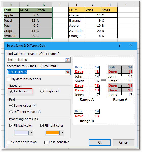
Compare two ranges

Now you know how to compare two columns after reading above methods. However, in some cases, you may want to compare two ranges (two series with multiple columns) You can use above methods (the formulas or conditional formatting) to compare them column by column, but here introduces a handy tool – Kutools for Excel can solve this job in different cases quickly with formula free.

• Example 1: Compare two ranges by cell
• Example 2: Compare two ranges if data in the same order

Example 1: Compare two ranges by cell

Here are two ranges needed to be compared by cells, you can use the Select Same & Different Cells utility of Kutools for Excel to handle it.

After free installing Kutools for Excel, click Kutools > Select > Select Same & Different Cells. Then in the popping Select Same & Different Cells dialog, do as below:

1. In the Find values in section, choose the range that you want to find out the matches or differences after comparing two ranges.
2. In the According to section, choose the other range used to compared range.
3. In Based on section, choose Single cell.
4. In the Find section, choose the type of cells that you want to select or highlight.
5. In the Processing of results section, you can highlight the cells by fill background color or the font color, if you do not need to highlight, do not tick the checkboxes. Click OK.

A dialog pops out and reminds how many cells/rows have been selected, click OK to close it.

• Selecting and highlight the unique values
  
• Selecting and highlighting the duplicate values
  

Example 2: Compare two ranges if data in the same order

Supposing, the range F2:H7 is a model, now you want to find if the data in range B2:D7 is in the right order according to the range F2:H7.

In this case, the Compare Cells of Kutools for Excel can help you.

After free installing Kutools for Excel, click Kutools > Compare Cells. Then in the Compare Cells dialog, set as below:

1. Choose the two ranges into the Find values in and According to boxes separately.
2. Choose the cell type that you want to highlight in the Find section.
3. Choose the highlighting type in the Processing of results section. Click OK.

A dialog pops out and reminds how many cells have been selected, click OK to close it. Now the cells that are different with those in the other range have been selected and highlighted.

The information provided above details how to compare columns in Excel. I hope you find it valuable and beneficial. For more invaluable Excel tips and tricks that can transform your data processing, dive in here.