How to fill drop-down list cells with only colors and not texts in Excel?
When managing information such as project status in Excel, it's common to use drop-down lists accompanied by stoplight colors—such as Green for "good", Yellow for "at risk", and Red for "off track". Using visual color cues makes status reporting more accessible and immediate, especially in project oversight, task management, and dashboards. In many cases, you may prefer to keep cells visually simple by displaying only color, without text, for a more streamlined look. Achieving this typically requires combining cell formatting techniques. This article explores several practical methods to accomplish this purpose—from built-in Excel features to add-in solutions and advanced alternatives—so you can choose an approach that matches your workflow and needs.

Fill drop-down cells with colors and not texts with conditional formatting
Fill drop-down cells with colors and not texts with an amazing tool
Fill drop-down cells with colors and not texts with conditional formatting
Excel’s built-in conditional formatting helps visually distinguish values in drop-down lists by assigning colors to different project or task statuses. However, while conditional formatting assigns colors based on cell values, the cell text still remains visible by default. To display only color and hide the text, you need to set up a custom cell format.
Important: Hiding the cell value using custom formatting means the text is not visible in the worksheet, but it still exists in the cell. If you later need to review the status as text, you can temporarily remove the custom format.
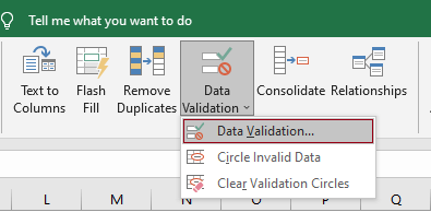
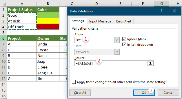
1. Firstly, you need to create a drop-down list in cells of the Status column.
Note: If you have created the drop-down list in the cells, skip this step.
2. Keeping the drop-down cells selected, go to Home > Conditional Formatting > Highlight Cells Rules > Equal To.

3. In the Equal To dialog box, configure as follows.

4. In the Format Cells dialog, under the Fill tab, pick a color to represent the status. Click OK to confirm.

5. Click OK to finalize the rule and return to the Equal To dialog.
6. Repeat steps 2 – 5 for each different status value in your drop-down list, assigning specific colors as needed. For larger lists, you may use a "New Rule" and "Use a formula" for more complex conditions and color coding.
By default, when a value is selected from the drop-down, both the color and text will be visible. To display only the color, follow these additional steps.

7. Select the drop-down list cells, right-click and choose Format Cells from the context menu.

8. In the Format Cells dialog under the Number tab:

After these steps, your drop-down cells will visually display only the color. The text remains in the cell (for formulas or calculations), but is hidden from view. To restore text visibility, simply clear the custom format.
Fill drop-down cells with colors and not texts with an amazing tool
Setting up individual conditional formatting rules for every drop-down value can be tedious, especially in workbooks with many different lists or status categories. To quickly assign colors and control drop-down appearance, you can utilize the Colored Drop-down List feature available in Kutools for Excel. This tool streamlines the process, allowing you to easily match colors to drop-down choices and then hide cell text through formatting, ensuring a clean and intuitive worksheet layout.
1. Select the cells containing drop-down lists where you want to assign colors for each status or category.
2. Go to Kutools > Drop-down List > Colored Drop-down List.

3. In the Colored Drop-down list dialog:

All drop-down entries in your selected range now display the assigned colors. To show only colors in cells and hide the text, follow these steps:
4. Select the colored drop-down cells, right-click, and pick Format Cells.

5. In the Format Cells dialog box, under the Number tab:

Your drop-down list cells now feature only background colors, with text hidden from the view—ideal for dashboards and summary visuals.
Kutools for Excel - Supercharge Excel with over 300 essential tools, making your work faster and easier, and take advantage of AI features for smarter data processing and productivity. Get It Now
Best Office Productivity Tools
Supercharge Your Excel Skills with Kutools for Excel, and Experience Efficiency Like Never Before. Kutools for Excel Offers Over 300 Advanced Features to Boost Productivity and Save Time. Click Here to Get The Feature You Need The Most...
Office Tab Brings Tabbed interface to Office, and Make Your Work Much Easier
- Enable tabbed editing and reading in Word, Excel, PowerPoint, Publisher, Access, Visio and Project.
- Open and create multiple documents in new tabs of the same window, rather than in new windows.
- Increases your productivity by 50%, and reduces hundreds of mouse clicks for you every day!
All Kutools add-ins. One installer
Kutools for Office suite bundles add-ins for Excel, Word, Outlook & PowerPoint plus Office Tab Pro, which is ideal for teams working across Office apps.
- All-in-one suite — Excel, Word, Outlook & PowerPoint add-ins + Office Tab Pro
- One installer, one license — set up in minutes (MSI-ready)
- Works better together — streamlined productivity across Office apps
- 30-day full-featured trial — no registration, no credit card
- Best value — save vs buying individual add-in