Compare Two Ranges in Excel: Find Matching or Non-Matching Values
There are many times in Excel when you need to compare one range with another to see which values match and which do not. This can be useful for checking entries against an approved list, spotting unexpected values, reviewing imported data, or validating information spread across multiple columns.
Excel does not offer a single built-in command for this kind of comparison, but you can still do it effectively with Conditional Formatting. If you want a more direct approach, Kutools for Excel provides a dedicated tool that can compare ranges and select the matching or non-matching results for you.
In this tutorial, we’ll walk through both methods so you can choose the one that works best for your worksheet and your workflow.
Find matching or non-matching values using Conditional Formatting
Conditional Formatting provides a built-in way to highlight values that appear in another range. It is a good choice when you want to compare ranges directly in Excel without using add-ins, and it can be adapted for both exact and partial match checks depending on the formula you use.
Step 1: Prepare your worksheet
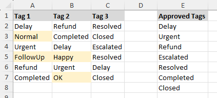
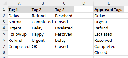
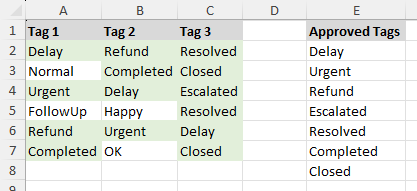
Set up your worksheet with:
- A data range containing the values you want to check, such as A1:C7.
- A reference range containing the values you want to compare against, such as E1:E8.
Note:
Both the data range and the reference range can contain either a single column or multiple columns.

Step 2: Create a rule to find matching values
- Select the range that contains the values you want to compare, such as A2:C7.
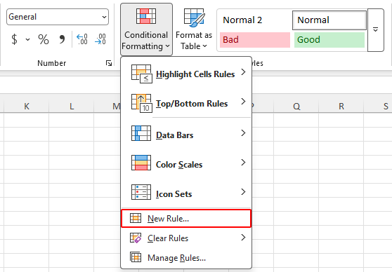
- Click Home > Conditional Formatting > New Rule.
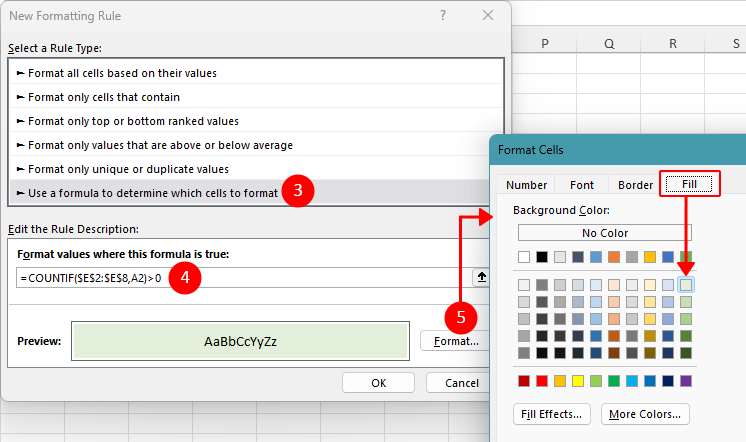
- Select Use a formula to determine which cells to format.
- Enter the following formula:
=COUNTIF($E$2:$E$8,A2)>0Note:
In the formula above, $E$2:$E$8 is the reference list, and A2 is the first cell in the selected range. Adjust the range references to match your worksheet.
- Click Format, choose the fill color you want, and click OK.
- Click OK again to apply the rule.


Excel will now highlight cells in the selected range whose values also appear in the reference list.
Step 3: Create a rule to find non-matching values
If you want to highlight values that do not appear in the reference list, use this formula instead:
=COUNTIF($E$2:$E$8,A2)=0Apply it the same way through Conditional Formatting.
Note:
The COUNTIF function evaluates all cells in the reference range for exact matches. To perform a partial match, modify the formula to use functions like SEARCH instead of exact matching. For example, the below formula highlights a cell if it contains any text from the reference list.
=SUMPRODUCT(--($E$2:$E$8<>""),--ISNUMBER(SEARCH($E$2:$E$8,A2)))>0Pros
- Built into Excel with no add-ins required
- Offers flexible matching by letting you customize the formula to suit your data
- Good for quick visual validation
Cons
- Requires setting up formulas manually
- Less convenient for users unfamiliar with Conditional Formatting formulas
Select and highlight matching or non-matching values using Kutools for Excel
If you want a quicker and more flexible way to compare values between ranges, Kutools for Excel offers a dedicated feature called Select Same & Different Cells. It can not only find matching or non-matching values without formulas, but also select the results directly for further actions such as formatting, copying, or deleting. In addition to comparing individual cells, it can also identify entire matching or non-matching rows.
Step 1: Open the Select Same & Different Cells feature
After installing Kutools for Excel, click Kutools > Select > Select Same & Different Cells.
Step 2: Set the options to find matching or non-matching values
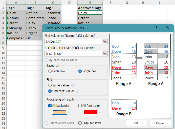
- Select the first range that contains the values you want to compare in the Find values in box.
- Select the comparison range in the According to box.
- Choose Single cell under Based on.
- Choose Same values if you want to find matches, or choose Different values if you want to find non-matching cells.
- Specify a fill color or font color to have the results highlighted directly.
- Click OK.

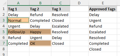
Kutools will immediately select and optionally highlight the cells whose values match or do not match the comparison range.
Notes:
- This method is intended for exact matches. If a cell contains longer text and only part of it matches a value in the comparison range, it will not be treated as a match.
- Both the selected range and the comparison range can contain one or multiple columns.
- You can check the Case Sensitive option to make the comparison distinguish between uppercase and lowercase letters. For example, Excel and excel will be treated as different values.
Pros
- No formulas are needed
- Selects matching or non-matching results directly for further actions
- Supports both cell-by-cell and row-by-row comparison
- Provides a faster and more visual way to compare ranges
Cons
- Requires Kutools for Excel
- Works with exact cell matches, not partial text matches
Kutools for Excel - Packed with over 300 essential tools for Excel. Make Excel tasks faster, easier, and more efficient. Download now!
Which method works best for you?
| Method | Best for | Limitations |
|---|---|---|
| Conditional Formatting | Highlighting matching or non-matching values with a built-in Excel feature | Requires formulas and manual setup |
| Kutools for Excel | Quickly selecting matching or non-matching cells or rows for further actions, without writing formulas | Requires Kutools for Excel Download |
Conclusion
If you want to highlight matching or non-matching values with a built-in Excel feature, Conditional Formatting is a solid choice. It gives you flexible control through formulas and can be adapted for both exact and partial match checks.
If you prefer a quicker and more direct method, Kutools for Excel makes the job easier. Its Select Same & Different Cells feature can compare ranges, select the results directly, and help you take further actions right away.
I hope you found this tutorial helpful. If you’d like to explore more Excel tips and practical solutions, please click here to browse our full collection of Excel tutorials.
The Best Office Productivity Tools
Kutools for Excel - Helps You To Stand Out From Crowd
Kutools for Excel Boasts Over 300 Features, Ensuring That What You Need is Just A Click Away...
Office Tab - Enable Tabbed Reading and Editing in Microsoft Office (include Excel)
- One second to switch between dozens of open documents!
- Reduce hundreds of mouse clicks for you every day, say goodbye to mouse hand.
- Increases your productivity by 50% when viewing and editing multiple documents.
- Brings Efficient Tabs to Office (include Excel), Just Like Chrome, Edge and Firefox.
Table of Contents
- Highlight using Conditional Formatting
- Select and highlight using Kutools for Excel
- Which method works best for you?
- Conclusion
- The Best Office Productivity Tools
Kutools for Excel
Brings 300+ advanced features to Excel
- 🧩 Overview
- 📥 Free Download
- 🎁 30-Day Free Trial available