Combine duplicate rows and sum their values in Excel (Simple Tricks)
In Excel, it's a common scenario to encounter a dataset with duplicate entries. Often, you might find yourself with a range of data where the key challenge is to efficiently combine these duplicate rows while simultaneously summing up the values in a corresponding column as following screenshot shown. In this context, we'll delve into several practical methods that can help you consolidate duplicate data and aggregate their associated values, enhancing both the clarity and utility of your Excel workbooks.
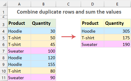
Combine duplicate rows and sum the values
Combine duplicate rows and sum the values with the Consolidate function
The Consolidate is a useful tool for us to consolidate multiple worksheets or rows in Excel, with this feature, we can combine duplicate rows and sum up their corresponding values quickly and easily. Please do with the following steps:
Step 1: Select a Destination Cell
Choose where you want the consolidated data to appear.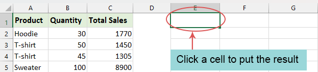
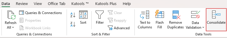
Step 2: Access the Consolidate Function and set up the consolidation
- Click "Data" > "Consolidate", see screenshot:
- In the "Consolidate" dialog box:
- (1.) Select "Sum" from "Function" drop down list;
- (2.) Click to select the range that you want to consolidate in the "Reference" box;
- (3.) Check "Top row" and "Left column" from "Use labels in" option;
- (4.) Finally, click "OK" button.


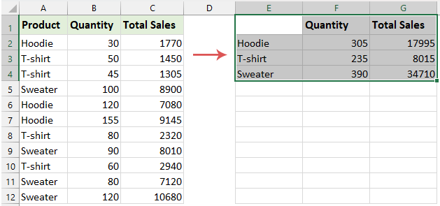
Result:
Excel will combine any duplicates found in the first column and sum their corresponding values in the adjacent columns as following screenshot shown:
- If the range doesn't include a header row, ensure to "uncheck Top row" from the "Use labels in" option.
- With this feature, calculations can only be consolidated based on the first column (the leftmost one) of the data.
Use Kutools to combine duplicate rows and sum the values
If you have installed "Kutools for Excel", its "Advanced Combine Rows" feature allows you to easily combine duplicate rows, providing options to sum, count, average, or execute other calculations on your data. Moreover, this feature isn't limited to just one key column, it can handle multiple key columns, making complex data consolidation tasks much easier.
After installing "Kutools for Excel", select the data range, and then click "Kutools" > "Merge & Split" > "Advanced Combine Rows".
In the "Advanced Combine Rows" dialog box, please set the following operations:
- Click the column name that you want to combine duplicates based on, here, I will click Product, and then select "Primary Key" from the drop-down list in the "Operation" column;
- Then, select the column name you want to sum the values, and then select "Sum" from the drop-down list in the "Operation" column;
- As for the other columns, you can choose the operation you need, such as combining the values with a specific separator or performing a certain calculation; (this step can be ignored if you have only two columns)
- At last, you can preview the combined result then click "OK" button.


Result:
Now, the duplicate values in the key column are combined, and other corresponding values are summed up as following screenshot shown:

- With this useful feature, you can also combine rows based on duplicate cell value as following demo shown:

- This feature "supports Undo", if you want to recover your original data, just press "Ctrl + Z".
- To apply this feature, please download and install Kutools for Excel.

Use Pivot Table to combine duplicate rows and sum the values
Pivot Tables in Excel provide a dynamic way to rearrange, group, and summarize data. This functionality becomes incredibly useful when you are faced with a dataset filled with duplicate entries and need to sum corresponding values.
Step 1: Creating a Pivot Table
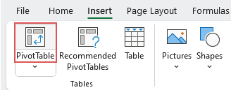
- Select the data range. And then, go to the "Insert" tab, and click "Pivot Table", see screenshot:
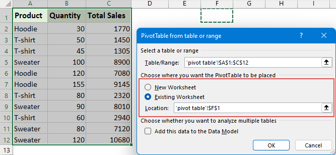
- In the popped-out dialog box, choose where you want the Pivot Table report to be placed, you can put it to a new sheet or existing sheet as you need. Then, click "OK". See screenshot:
- Now, a Pivot Table is inserted in the selected destination cell. See screenshot:


Step 2: Configuring the Pivot Table:
- In the "PivotTable Fields" pane, drag the field containing duplicates to the "Row" area. This will group your duplicates.
- Next, drag the fields with the values you want to sum to the "Values" area. By default, Excel sums the values. See the demo below:

Result:
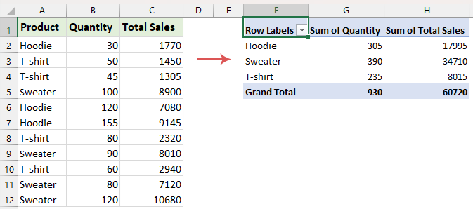
The Pivot Table now displays your data with duplicates combined and their values summed up, offering a clear and concise view for analysis. See screenshot:
Use VBA code to combine duplicate rows and sum the values
If you are interested in VBA code, in this section, we will give a VBA code to consolidate duplicate rows and sum the corresponding values in other columns. Please do with the following steps:
Step 1: Open the VBA sheet module editor and copy the code
- Hold down the "ALT + F11" keys in Excel to open the "Microsoft Visual Basic for Applications" window.
- Click "Insert" > "Module", and paste the following code in the "Module" Window.
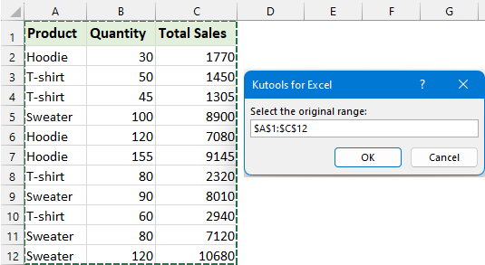
VBA code: Combine duplicate rows and sum the valuesSub CombineDuplicateRowsAndSumForMultipleColumns() 'Update by Extendoffice Dim SourceRange As Range, OutputRange As Range Dim Dict As Object Dim DataArray As Variant Dim i As Long, j As Long Dim Key As Variant Dim ColCount As Long Dim SumArray() As Variant Dim xArr As Variant Set SourceRange = Application.InputBox("Select the original range:", "Kutools for Excel", Type:=8) If SourceRange Is Nothing Then Exit Sub ColCount = SourceRange.Columns.Count Set OutputRange = Application.InputBox("Select a cell for output:", "Kutools for Excel", Type:=8) If OutputRange Is Nothing Then Exit Sub Set Dict = CreateObject("Scripting.Dictionary") DataArray = SourceRange.Value For i = 1 To UBound(DataArray, 1) Key = DataArray(i, 1) If Not Dict.Exists(Key) Then ReDim SumArray(1 To ColCount - 1) For j = 2 To ColCount SumArray(j - 1) = DataArray(i, j) Next j Dict.Add Key, SumArray Else xArr = Dict(Key) For j = 2 To ColCount xArr(j - 1) = xArr(j - 1) + DataArray(i, j) Next j Dict(Key) = xArr End If Next i OutputRange.Resize(Dict.Count, ColCount).ClearContents i = 1 For Each Key In Dict.Keys OutputRange.Cells(i, 1).Value = Key For j = 1 To ColCount - 1 OutputRange.Cells(i, j + 1).Value = Dict(Key)(j) Next j i = i + 1 Next Key Set Dict = Nothing Set SourceRange = Nothing Set OutputRange = Nothing End Sub
Step 2: Execute the code
- After pasting this code, please press "F5" key to run this code. In the prompt box, select the data range that you want to combine and sum. And then, click "OK".
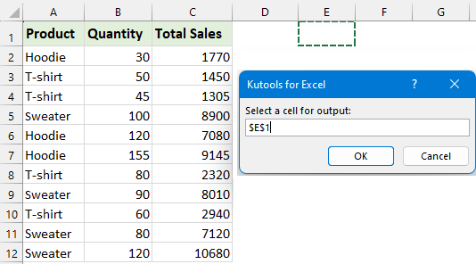
- And in the next prompt box, select a cell where you will output the result, and click "OK".


Result:
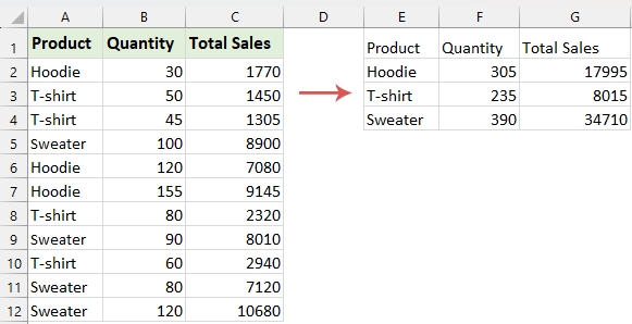
Now, the duplicate rows are merged, and their corresponding values have been summed up. See screenshot:
Combining and summing duplicate rows in Excel can be simple and efficient. Choose from the easy Consolidate function, the advanced Kutools, the analytical Pivot Tables, or the flexible VBA coding to find a solution that suits your skills and needs. If you're interested in exploring more Excel tips and tricks, our website offers thousands of tutorials, please click here to access them. Thank you for reading, and we look forward to providing you with more helpful information in the future!
Related Articles:
- Combine multiple rows into one based on duplicates
- Maybe, you have a range of data, in the Product name column A, there are some duplicate items, and now you need to remove the duplicate entries in column A but combine the corresponding values in column B.How could aove this task in Excel?
- Vlookup and return multiple values without duplicates
- Sometimes, you may want to vlookup and return multiple matched values into a single cell at once. But, if there are some repeated values populated into the returned cells, how could you ignore the duplicates and only keep the unique values when returning all matching values as following screenshot shown in Excel?
- Combine rows with same ID/name
- For example, you have a table as below screenshot shown, and you need to combine rows with the order IDs, any ideas? Here, this article will introduce two solutions for you.
Best Office Productivity Tools
Supercharge Your Excel Skills with Kutools for Excel, and Experience Efficiency Like Never Before. Kutools for Excel Offers Over 300 Advanced Features to Boost Productivity and Save Time. Click Here to Get The Feature You Need The Most...
Office Tab Brings Tabbed interface to Office, and Make Your Work Much Easier
- Enable tabbed editing and reading in Word, Excel, PowerPoint, Publisher, Access, Visio and Project.
- Open and create multiple documents in new tabs of the same window, rather than in new windows.
- Increases your productivity by 50%, and reduces hundreds of mouse clicks for you every day!
All Kutools add-ins. One installer
Kutools for Office suite bundles add-ins for Excel, Word, Outlook & PowerPoint plus Office Tab Pro, which is ideal for teams working across Office apps.
- All-in-one suite — Excel, Word, Outlook & PowerPoint add-ins + Office Tab Pro
- One installer, one license — set up in minutes (MSI-ready)
- Works better together — streamlined productivity across Office apps
- 30-day full-featured trial — no registration, no credit card
- Best value — save vs buying individual add-in