Excel Checkboxes: Add, select, delete and use checkboxes in Excel
A checkbox is an interactive tool used to select or deselect an option. You will often see them on web forms or when filling in surveys. In Excel, you can add manifold possibilities by checking or unchecking a checkbox, making your sheet more dynamic and interactive. For example, you can create checklists, insert dynamic charts, etc.
In this tutorial, I will explain how to insert, select, and delete checkboxes, along with some examples of how to use them in Excel.
Table of contents:
1. Two types of checkboxes (Check Box Form control vs. Check Box ActiveX control)
2. Add one or multiple checkboxes in Excel
3. Change the checkbox name and caption text
4. Link one or multiple checkboxes to cells
5. Select one or multiple checkboxes
6. Delete one or multiple checkboxes
8. Examples: How to use checkboxes in Excel
- Example 1: Create To-do list with checkboxes
- Example 2: Create dynamic chart with checkboxes
- Example 3: Create drop-down list with checkboxes
- Example 4: Check checkbox to change row color
- Example 5: Count or sum cell values if the checkbox is checked
- Example 6: If checkbox is checked then return a specific value
Two types of checkboxes (Check Box Form control vs. Check Box ActiveX control)
To insert a checkbox, you need to make sure that the Developer tab is visible on the ribbon. The Developer tab is not active by default, so you need to enable it firstly.
1. In the Excel workbook, please click File > Options. In the Excel Options dialog box, click Customize Ribbon, then check Developer option and click OK button to close this dialog.

2. Now, the Developer tab appears in the Excel ribbon as below screenshot shown. You can access a variety of interactive controls from the Developer tab as you need.

Microsoft Excel provides two types of checkbox-Check Box Form control and Check Box ActiveX control:
 |  |
Check Box Form Control is much simpler than Check Box ActiveX Control, and the Check Box ActiveX Control is more flexible in design and can be used as objects in codes. For our daily work, the Form Controls are sufficient, so we will use them in most cases.
Check Box Form control vs. Check Box ActiveX control:
- ActiveX controls provide more formatting options, you can use them for a sophisticated and flexible design;
- Form controls are built into Excel while ActiveX controls are loaded separately, so they may freeze occasionally;
- Some computers don't trust ActiveX controls by default, so you need to enable them manually from the Trust Center;
- Check Box ActiveX control can be accessed programmatically via the VBA editor;
- ActiveX is only provided by Windows option, and Mac OS doesn't support it.
Note: All the checkboxes I talk about in the following tutorials are Check Boxes Form Control.
Add one or multiple checkboxes in Excel
To insert one or more checkboxes, this section may do you a favor.
2.1 Insert one checkbox
To insert a checkbox, please do as this:
1. Click Developer tab, then click Insert from the Controls group, and then select Check Box under Form Controls. Then, click a cell where you want to insert the checkbox, and the checkbox will appear near that cell, see screenshots:

2. Then, put your cursor over the edge of the selection box for your checkbox. When it changes to the move pointer, you can click and drag the checkbox into the cell you need, see screenshots:

2.2 Insert multiple checkboxes
If you need multiple checkboxes in your worksheet, here will talk about some quick ways for you.
Insert multiple checkboxes with Fill Handle option
To insert multiple checkboxes quickly, add one checkbox as described above, and then use the Fill Handle option to fill the checkboxes to other cells.
1. Click to select the cell where the checkbox located.
2. Drag the fill handle down to fill the checkboxes as below screenshot shown:

Insert multiple checkboxes with VBA code
The following VBA code also can help you to insert a list of checkboxes quickly and easily. Please do as this:
1. Hold down the ALT + F11 keys to open the Microsoft Visual Basic for Applications window.
2. Then, click Insert > Module, and paste the following code in the Module window.
VBA code: Insert multiple checkboxes into a list of cells
Sub InsertCheckBoxes()
'Update by Extendoffice
Dim Rng As Range
Dim WorkRng As Range
Dim Ws As Worksheet
On Error Resume Next
xTitleId = "KutoolsforExcel"
Set WorkRng = Application.Selection
Set WorkRng = Application.InputBox("Range", xTitleId, WorkRng.Address, Type:=8)
Set Ws = Application.ActiveSheet
Application.ScreenUpdating = False
For Each Rng In WorkRng
    With Ws.CheckBoxes.Add(Rng.Left, Rng.Top, Rng.Width, Rng.Height)
        .Characters.Text = Rng.Value
    End With
Next
WorkRng.ClearContents
WorkRng.Select
Application.ScreenUpdating = True
End Sub
3. Press F5 key to run this code. A prompt box will pop out to remind you to select a range of cells for inserting the checkboxes. See screenshot:

4. Then, click OK button, the checkboxes are neatly inserted into the cells at once. See the screenshot:

Insert multiple checkboxes with a handy feature
If you have Kutools for Excel, with its Batch Insert Smart Checkboxes feature, you can insert the checkboxes into blank cells or cells with data immediately.
1. Select a range of cells where you want to insert checkboxes.
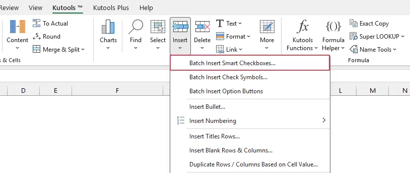
2. Then, click Kutools > Insert > Batch Insert Smart Checkboxes, see screenshot:
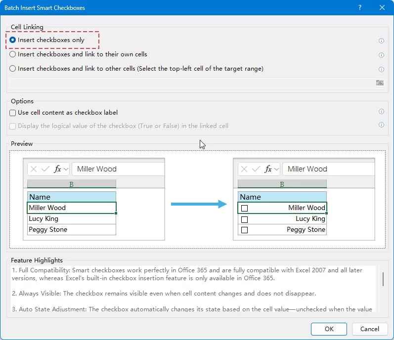
3. In the Batch Insert Smart Checkboxes dialog box, select Insert Chekboxes only option from the Cell Linking section, see screenshot:
4. And then, click OK. the selected cells are filled with checkboxes as following screenshots shown:
| Insert checkboxes into blank cells | Insert checkboxes into data cells |
 |  |
Kutools for Excel - Supercharge Excel with over 300 essential tools, making your work faster and easier, and take advantage of AI features for smarter data processing and productivity. Get It Now
Change the checkbox name and caption text
When using a checkbox in Excel, you should distinguish between the checkbox name and caption name. The caption name is the text you see beside the checkbox, and the checkbox name is the name you see in the Name box when the checkbox is selected as below screenshots shown:
| Checkbox name | Caption name |
 |  |
To change the caption name, please right click the checkbox, and then select Edit Text from the context menu, and type the new name you want, see screenshots:

To change the checkbox name, you should select the checkbox, and then enter the name you need into the Name box as below screenshot shown:

Link one or multiple checkboxes to cells
When using the checkbox, you often need to link the checkboxes to cells. If the box is checked, the cell shows TRUE, and if unchecked, the cell shows FALSE or empty. This section will introduce how to link one or multiple checkboxes to cells in Excel.
4.1 Link one checkbox to a cell with Format Control feature
To associate the checkbox with a certain cell, please do as this:
1. Right click the checkbox, and then select Format Control from the context menu, see screenshot:

2. In the Format Object dialog box, under the Control tab, click to select a cell where you want to link to the checkbox from the Cell link box, or type the cell reference manually, see screenshot:

3. Click OK to close the dialog box, and now, the checkbox is linked to a specific cell. If you check it, a TRUE is displayed, uncheck it, a FALSE is appeared as below demo shown:

4.2 Link multiple checkboxes to cells with VBA code
To link multiple checkboxes to cells by using the Format Control feature, you need to repeat the above steps again and again. This will be time-consuming if there are hundreds or thousands of checkboxes needed to be linked. Here, I will introduce a VBA code to link multiple checkboxes to cells at once.
1. Go to the worksheet which contains the checkboxes.
2. Hold down the ALT + F11 keys to open the Microsoft Visual Basic for Applicationswindow.
3. Then, click Insert > Module, and paste the following code in the Module Window.
VBA code: Link multiple checkboxes to cells at once
Sub LinkChecks()
'Update by Extendoffice
Dim xCB
Dim xCChar
i = 2
xCChar = "C"
For Each xCB In ActiveSheet.CheckBoxes
If xCB.Value = 1 Then
    Cells(i, xCChar).Value = True
Else
    Cells(i, xCChar).Value = False
End If
xCB.LinkedCell = Cells(i, xCChar).Address
i = i + 1
Next xCB
End Sub
Note: In this code, i = 2, the number 2 is the starting row of your checkbox, and xCChar = "C", the letter C is the column where you want to link the checkboxes to. You can change them to your need.
4. Press F5 key to run this code. All checkboxes in the active worksheet are linked to the specified cells at once. When checking a checkbox, its relative cell will display TRUE, unchecking the checkbox, the linked cell will show FALSE, see screenshot:

4.3 Link multiple checkboxes to cells with Kutools
Kutools for Excel makes this process much easier because you do not need to set the cell link for each checkbox manually. It allows you to handle multiple checkboxes at once, which is especially helpful when creating large checklists, forms, or worksheet controls.
This method is faster, easier, and more practical than manually editing each checkbox property one by one.
1. Select the cells where you want to insert checkboxes, with each checkbox linked to a corresponding cell.
2. Click Kutools > Insert > Batch Insert Smart Checkboxes.
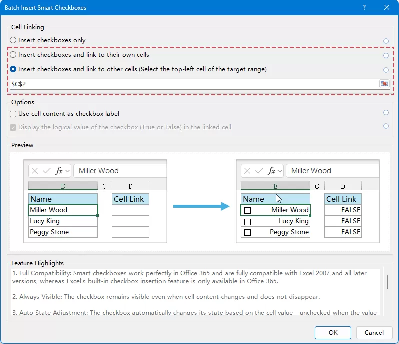
3. In the Batch Insert Checkboxes dialog box, choose the option for linking checkboxes to cells:
- Select Insert checkboxes and link to their own cells to link each checkbox to the cell where it is inserted.
- Select Insert checkboxes and link to other cells (Select the top-left cell of the target range), and then choose a blank cell as the starting cell for the linked-cell range. In this example, select $C$2. The checkbox results will be linked to the cells starting from C2.

4. Click OK to insert the checkboxes and create the linked cells.
| Insert checkboxes and link to their own cells | Insert checkboxes and link to other cells |
 |  |
Select one or multiple checkboxes
To copy or delete the checkboxes in a worksheet, you should select the checkboxes first. To select one or more checkboxes, please do as this:
Select a single checkbox: (two ways)
- Right click the checkbox, and then click anywhere within it.
- OR
- Press the Ctrl key, and then click on the checkbox.
Select multiple checkboxes:
Press and hold the Ctrl key, and then click on the checkboxes you want to select one by one.
Delete one or multiple checkboxes
Deleting one checkbox is easy for us, you just need to select it and then press Delete key on your keyboard. When it comes to multiple checkboxes, how could you do it in Excel?
6.1 Delete multiple checkboxes with VBA code
For deleting all checkboxes within a sheet, you can apply the following VBA code.
1. Hold down the ALT + F11 keys to open the Microsoft Visual Basic for Applications window.
2. Then, click Insert > Module, and paste the following code in the Module window.
VBA code: Delete all checkboxes in current worksheet
Sub RemoveCheckboxes()
'Update by Extendoffice
On Error Resume Next
ActiveSheet.CheckBoxes.Delete
Selection.FormatConditions.Delete
End Sub
3. Then, press F5 key to execute the code. All checkboxes in the specific worksheet will be deleted at once.
6.2 Delete multiple checkboxes with a simple feature
With Kutools for Excel’s Batch Delete Check Boxes feature, you can delete checkboxes from a selected range or entire sheets with just a few clicks.
1. Select the range of cells or the entire sheet which contain checkboxes you want to remove.
2. Then, click Kutools > Delete > Batch Delete Check Boxes, see screenshot:

3. And then, all checkboxes are removed at once from the selection.
Group checkboxes in Excel
When you want to move or resize multiple checkboxes together, grouping the checkboxes may help to control on all checkboxes at once. This section will talk about how to group multiple checkboxes in an Excel worksheet.
7.1 Group checkboxes by using Group feature
In Excel, the Group feature can help to group multiple checkboxes, please do as this:
1. Hold the Ctrl key, and then click to select the checkboxes one by one that you want to group, see screenshot:

2. Then, right click and choose Group > Group from the context menu, see screenshot:

3. Once all selected checkboxes are grouped, you can move or copy them together at once.

7.2 Group checkboxes by using Group Box Command
Additionally, you can also use the Group Box to group multiple checkboxes together. Please do with the following steps:
1. Go to the Developer tab, and then click Insert > Group Box (Form Control), see screenshot:

2. And then, drag the mouse to draw a group box, and change the group box caption name as you like:
 |  |
3. Now, you can insert checkboxes into the group box, click Developer > Insert > Check Box (Form Control), see screenshot:

4. Then drag the mouse to draw a checkbox, and modified the caption name as you need, see screenshots
 |  |
5. Similarly, insert other checkboxes into the group box and you will get the result as below screenshot shown:

Examples: How to use checkboxes in Excel
From above information, we know some basic knowledge of the checkboxes. In this section, I will introduce how to use checkboxes for some interactive and dynamic operations in Excel.
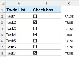
Example 1: Create To-do list with checkboxes
A To-do list is useful for marking tasks that have been completed in our daily work. In a typical To-do list, the checked completed tasks have the strikethrough format like the below screenshot shown. With the help of checkboxes, you can create an interactive To-do list quickly.

To create a To-do list with checkboxes, please with the following steps:
1. Please insert the checkboxes into the list of cells where you want to use, see screenshot: (Click to know how to insert multiple checkboxes)

2. After inserting the checkboxes, you should link each checkbox to a separate cell.
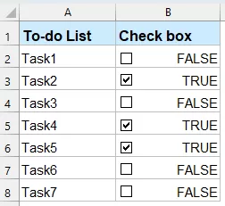
3. After linking checkboxes to cells, if the checkbox is checked, a TRUE is displayed, if unchecked, a FALSE is displayed, see screenshot:

4. ext, apply the Conditional Formatting feature to perform the following steps. Select the cell range A2:C8 that you want to create a To -do list, and then click Home > Conditional Formatting > New Rule to go to the New Formatting Rule dialog box.
5. In the New Formatting Rule dialog, click Use a formula to determine which cells to format in the Select a Rule Type list box, and then enter this formula =C2=TRUE into the Format values where this formula is true text box, see screenshot:
Note: C2 is a cell which linked to the checkbox..

6. Then, go on clicking the Format button to go to the Format Cells dialog box. Under the Font tab, check the Strikethrough from the Effects section, and specify a color for the completed to do list item as you want, see screenshot:

7. Then, click OK > OK to close the dialogs, now, when you check the check box, its corresponding item will be formatted as strikethrough as below demo shown:

Example 2: Create dynamic chart with checkboxes
Sometimes, you may need to display a lot of data and information in one chart, and the chart will be in mess. In this case, you can use checkboxes to create a dynamic chart in your sheet. When you check a checkbox, the corresponding data line will be displayed; if unchecked, the data line will be hidden, as shown in the demo below.

This section will talk about two quick tricks for creating this type of chart in Excel.
Create interactive chart with checkboxes in Excel
Normally, in Excel, you can create a dynamic chart by using checkboxes with following steps:
1. Insert some checkboxes and rename them. In this case, I will insert three checkboxes and rename them as Apple, Orange, and Peach, as shown in the screenshot::

2. Then, you should link these checkboxes to cells, please click to select the first checkbox, and then right click, then choose Format Control, in the Format Object dialog box, under the Control tab, from the Cell link box, select a cell where to link with the checkbox, see screenshot:

3. Repeat the above step to link the other two checkboxes to different cells. Now, if you check the checkbox, a TRUE will be shown, otherwise, a FALSE will be displayed as below demo shown:

4. After inserting and linking the checkboxes, now, you should prepare the data. Copy the original data row and column headings to another place, see screenshot:

5. Then apply the below formulas:
- In cell B13: =IF($B$6,B2,NA()), and drag the fill handle to fill the row from B13 to G13;
- In cell B14: =IF($B$7,B3,NA()),and drag the fill handle to fill the row from B14 to G14;
- In cell B15: =IF($B$8,B4,NA()),and drag the fill handle to fill the row from B15 to G15.
- These formulas return values from the original data if the checkbox for that product is checked, and #N/A if it is unchecked. See screenshot:

6. Then, please select the new data range from A12 to G15, and then, click Insert > Insert Line or Area Chart > Line to insert a line chart.
7. Now, when you check the product checkbox, its data line will appear, and when uncheck, it will disappear as below demo shown:

8. After creating the chart, then, you can place the checkboxes onto the chart to make them look neat. Click to select the plot area, and then drag to shrink it, see screenshot:

9. Press Ctrl key to select the three checkboxes, drag them onto the chart, then, right click to choose Bring to Front > Bring to Front, see screenshot:

10. And the checkboxes are displayed onto the chart, go on pressing Ctrl key to select the checkboxes and chart one by one, right click to select Group > Group, see screenshot:

11. Now, the checkboxes are linked with the line chart. When you move the chart, the checkboxes will also move accordingly.

Create interactive chart with checkboxes with an easy feature
The above method may be somewhat difficult for you, here, I will introduce an easy way for solving this task. With Kutools for Excel’s Check Box Line Chart feature, you can create a dynamic chart with checkboxes with ease.
1. Select the data range that you want to create the chart, and then click Kutools > Charts > Category Comparison > Check Box Line Chart, see screenshot:

2. And then, a Check Box Line Chart dialog box is popped out, the selected data is automatically filled into separate textboxes. See the screenshot:

3. Then, click OK button, and a prompt box is popped out to remind you a hidden sheet with some intermediate data will be created, please click Yes button, see screenshot:

4. And a line chart with checkboxes will be created successfully, see screenshot:

Kutools for Excel - Supercharge Excel with over 300 essential tools, making your work faster and easier, and take advantage of AI features for smarter data processing and productivity. Get It Now
Example 3: Create drop-down list with checkboxes
Selecting multiple items from a drop-down list is a common task for many users. Some users try to create a drop-down list with checkboxes to choose multiple selection as below demo shown. Unfortunately, Excel does not natively support creating drop-down lists with checkboxes. But here, I will introduce two types of multiple checkboxes selection in Excel. One is a list box with checkboxes, and another is a drop-down list with checkboxes.
Create drop-down list with checkboxes by using list box
Instead of a drop-down list, you can use a list box to add checkboxes for multiple selection. The process is a little complicated, please follow the below steps step by step:
1. First, please insert a List Box, click Developer > Insert > List Box (ActiveX Control). See screenshot:

2. Drag the mouse to draw a list box, and then right click it, choose Properties from the context menu, see screenshot:

3. In the Properties pane, please set the operations as follows:
- In the ListFillRange box, enter the data range you want to display in the list box;
- In the ListStyle box, select 1 - fmList StyleOption from the drop down;
- In the MultiSelect box, select 1 – fmMultiSelectMulti from the drop down;
- Finally, click close button to close it.

4. Then, click a cell where you want to output the multiple selected items, and give a range name for it. Please type a range name “Outputitem” into the Name box and press Enter key, see screenshot:

5. Next, click Insert > Shapes > Rectangle, then drag the mouse to draw a rectangle above the list box. See screenshot:

6. Right-click the rectangle and select Assign Macro from the context menu. See screenshot:

7. In the Assign Macro dialog, click New button, see screenshot:

8. In the opened Microsoft Visual Basic for Applications window, replace the original code in the Module window with the following VBA code:
Sub Rectangle1_Click()
'Updated by Extendoffice
Dim xSelShp As Shape, xSelLst As Variant, I, J As Integer
Dim xV As String
Set xSelShp = ActiveSheet.Shapes(Application.Caller)
Set xLstBox = ActiveSheet.ListBox1
If xLstBox.Visible = False Then
    xLstBox.Visible = True
    xSelShp.TextFrame2.TextRange.Characters.Text = "Pickup Options"
    xStr = ""
    xStr = Range("Outputitem").Value

    If xStr <> "" Then
         xArr = Split(xStr, ";")
    For I = xLstBox.ListCount - 1 To 0 Step -1
        xV = xLstBox.List(I)
        For J = 0 To UBound(xArr)
            If xArr(J) = xV Then
              xLstBox.Selected(I) = True
              Exit For
            End If
        Next
    Next I
    End If
Else
    xLstBox.Visible = False
    xSelShp.TextFrame2.TextRange.Characters.Text = "Select Options"
    For I = xLstBox.ListCount - 1 To 0 Step -1
        If xLstBox.Selected(I) = True Then
        xSelLst = xLstBox.List(I) & ";" & xSelLst
        End If
    Next I
    If xSelLst <> "" Then
        Range("Outputitem") = Mid(xSelLst, 1, Len(xSelLst) - 1)
    Else
        Range("Outputitem") = ""
    End If
End If
End Sub

Note: In the above code, Rectangle1 is the shape name, ListBox1 is the name of the list box, and the Outputitem is the range name of the output cell. You can change them based on your needs.
9. Then, close the code window. Now, clicking on the rectangle button will hide or display the list box. When the list box is displayed, select the items in the list box, and click the rectangle button again to output the selected items into the specified cell, see below demo:

Create drop-down list with checkboxes with an amazing feature
You can use the powerful Kutools for Excel to easily insert checkboxes into a real drop-down list. With its Drop-down List with Check Boxes feature, Kutools allows you to quickly create drop-down menus that support multiple selections with checkboxes—something that Excel doesn't support natively. This not only enhances the functionality of your lists but also significantly improves efficiency and user experience.
1. First, please insert the normal drop-down list in the selected cells, see screenshot:

2. click Kutools > Drop-down List > Enable Advanced Drop-down List. Then, click Drop-down List with Check Boxes from the Drop-down List again. See screenshot:

3. In the Add CheckBoxes to the Dropdown List dialog box, please configure as follows:
- 2.1) Select the cells containing the drop down list;
- 2.2) In the Separator box, enter a delimiter which you will use to separate the multiple items;
- 2.4) Click the OK button.


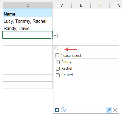
From now on, when you click a cell with a drop-down list, a list with check boxes will pop up, then select the items by checking the checkboxes to output the items into the cell as the below demo shown:
Example 4: Check checkbox to change row color
Have you ever tried to change the row color based on the checked checkbox? Which means the color of the related row will be changed if you check a checkbox as below screenshot shown, this section will talk about some tricks for solving this task in Excel.

Check checkbox to change cell color by using Conditional Formatting
To change the row color by checking or unchecking the checkbox, the Conditional Formatting feature in Excel can do you a favor. Please do as this:
1. First, insert the checkboxes into the list of cells as you need, see screenshot:

2. Next, you should link these checkboxes to the cells beside each checkbox separately, see screenshot:

3. Then, select the data range that you want to change row color, and then click Home > Conditional Formatting > New Rule, see screenshot:

4. In the New Formatting Rule dialog box, do the below operations:
- Select the Use a formula to determine which cells to format option in the Select a Rule Type box;
- Enter this formula =IF($F2=TRUE,TRUE,FALSE)into the Format values where this formula is true box;
- Click the Format button to specify a color you like for the rows.
Note: In the formula, $F2 is the first linked cell of the checkbox..

5. After choosing the color, click OK > OK to close the dialog boxes, and now, when you check a check box, the corresponding row will be highlighted automatically as bellow demo shown:

Check checkbox to change row color by using VBA code
The following VBA code also can help you to change the row color based on the checked checkbox, please do with the below code:
1. In the worksheet you want to highlight rows by checkboxes, right click the sheet tab and select View Code from the right-clicking menu. See screenshot:

2. Copy and paste the below code into the opened Microsoft Visual Basic for Applications window:
VBA code: Highlight rows by checking checkbox
Sub AddCheckBox()
Dim xCell As Range
Dim xRng As Range
Dim I As Integer
Dim xChk As CheckBox
On Error Resume Next
InputC:
    Set xRng = Application.InputBox("Please select the column range to insert checkboxes:", "Kutools for Excel", Selection.Address, , , , , 8)
If xRng Is Nothing Then Exit Sub
If xRng.Columns.Count > 1 Then
    MsgBox "The selected range should be a single column", vbInformation, "Kutools fro Excel"
    GoTo InputC
Else
    If xRng.Columns.Count = 1 Then
        For Each xCell In xRng
            With ActiveSheet.CheckBoxes.Add(xCell.Left, _
               xCell.Top, xCell.Width = 15, xCell.Height = 12)
               .LinkedCell = xCell.Offset(, 1).Address(External:=False)
               .Interior.ColorIndex = xlNone
               .Caption = ""
               .Name = "Check Box " & xCell.Row
            End With
            xRng.Rows(xCell.Row).Interior.ColorIndex = xlNone
        Next
    End If
    With xRng
     .Rows.RowHeight = 16
    End With
    xRng.ColumnWidth = 5#
    xRng.Cells(1, 1).Offset(0, 1).Select
    For Each xChk In ActiveSheet.CheckBoxes
      xChk.OnAction = "Sheet2.InsertBgColor"
    Next
End If
End Sub

Sub InsertBgColor()
Dim xName As Integer
Dim xChk As CheckBox
For Each xChk In ActiveSheet.CheckBoxes
  xName = Right(xChk.Name, Len(xChk.Name) - 10)
  If (xName = Range(xChk.LinkedCell).Row) Then
   If (Range(xChk.LinkedCell) = "True") Then
    Range("A" & xName, Range(xChk.LinkedCell).Offset(0, -2)).Interior.ColorIndex = 6
   Else
    Range("A" & xName, Range(xChk.LinkedCell).Offset(0, -2)).Interior.ColorIndex = xlNone
   End If
  End If
Next
End Sub
Note: In the above code, in this script xChk.OnAction = "Sheet2.InsertBgColor", you should change the sheet name-Sheet2 to your own (Sheet2 is the real name of the worksheet, you can get it from the left code window pane). See screenshot:

3. Then, put the cursor into the first part of the code, and press F5 key to run the code. In the popping up Kutools for Excel dialog box, please select the range you want to insert checkboxes, see screenshot:

4. Then, click OK button, the checkboxes are inserted into the selected cells as below screenshot shown:

5. From now on, if you check a checkbox, the relative row will be colored automatically as below screenshot shown:

Example 5: Count or sum cell values if the checkbox is checked
If you have a range of data with a list of checkboxes, now, you would like to count the number of the checked checkboxes or sum the corresponding values based on the checked checkboxes as below screenshot shown. How could you solve this task in Excel?

To solve this task, the important step is to link the checkboxes to relative cells beside the data. The checked checkbox will display TRUE in the linked cell, otherwise, a FALSE will be displayed, and then, you can use the count or sum function to get the result based on TRUE or FALSE value.
1. First, you should link the checkboxes to cells separately, if the checkbox is checked, a TRUE is displayed, if unchecked, a FALSE is displayed, see screenshot:

2. Then, apply the following formulas to count or sum the values based on the checked checkboxes:
Count values by checked checkboxes:
=COUNTIF(D2:D10,TRUE)
Note: In this formula, D2:D10 is the range of the link cells that you have set for the checkboxes.

Sum values by checked checkboxes:
=SUMPRODUCT(($D$2:$D$10=TRUE)*$C$2:$C$10)
Note: In this formula, D2:D10 is the range of the link cells that you have set for the checkboxes, and C2:C10 is the list of cells that you want to sum.

Example 6: If checkbox is checked then return a specific value
If you have a checkbox, when checking it, a specific value should be appeared in a cell, and when unchecking it, a blank cell is displayed as below demo shown:

To finish this job, please do as this:
1. First, you should link this checkbox to a cell. Right click the checkbox, and choose Format Control, in the popped out Format Object dialog box, under the Control tab, click to select a cell where you want to link with the checkbox from the Cell link box, see screenshot:

2. Then, click OK button to close the dialog box. Now, type this formula: =IF(A5=TRUE,"Extendoffice","") into a cell where you want to output the result, and then press Enter key.
Note: In this formula, A5 is the cell that linked to the checkbox, “Extendoffice” is the specific text, you can change them to your need.

3. Now, when you check the checkbox, the specific text will display, when uncheck it, a blank cell will show, see below demo:
Best Office Productivity Tools
Supercharge Your Excel Skills with Kutools for Excel, and Experience Efficiency Like Never Before. Kutools for Excel Offers Over 300 Advanced Features to Boost Productivity and Save Time. Click Here to Get The Feature You Need The Most...
Office Tab Brings Tabbed interface to Office, and Make Your Work Much Easier
- Enable tabbed editing and reading in Word, Excel, PowerPoint, Publisher, Access, Visio and Project.
- Open and create multiple documents in new tabs of the same window, rather than in new windows.
- Increases your productivity by 50%, and reduces hundreds of mouse clicks for you every day!
All Kutools add-ins. One installer
Kutools for Office suite bundles add-ins for Excel, Word, Outlook & PowerPoint plus Office Tab Pro, which is ideal for teams working across Office apps.
- All-in-one suite — Excel, Word, Outlook & PowerPoint add-ins + Office Tab Pro
- One installer, one license — set up in minutes (MSI-ready)
- Works better together — streamlined productivity across Office apps
- 30-day full-featured trial — no registration, no credit card
- Best value — save vs buying individual add-in