How to find the first, last or nth occurrence of a character in Excel?
In many data processing tasks, you may encounter lists of text strings containing special characters—such as the hyphen “-”—and need to determine the position of their first, last, or a specific (nth) occurrence. For instance, extracting information based on delimiters, analyzing part codes, or separating data components often requires pinpointing where a certain character appears within each string. However, Excel does not provide a direct built-in function to return the first, last, or nth occurrence position of a character in a cell. This article introduces several practical techniques and step-by-step solutions to accurately find these occurrences, supporting a variety of data parsing and preparation needs.
Find the last occurrence of character with formulas
Find the last occurrence of character with User Defined Function
Find the first or nth occurrence of character with formula
Find the first or nth occurrence of specific character with an easy feature
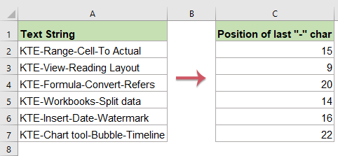
Find the last occurrence of character with formulas
If you want to return the position of the last occurrence of a specific character (such as “-”) in a text string, Excel’s standard functions do not provide this directly. However, by combining a few formulas, you can solve this problem efficiently. Here are two formula approaches, useful when dealing with product codes, file paths, or other data that follows a consistent separator pattern. Be aware that complex formulas may increase calculation load on large datasets.
1. In a blank cell (for example, C2), enter or copy one of the following formulas:
=SEARCH("^^",SUBSTITUTE(A2,"-","^^",LEN(A2)-LEN(SUBSTITUTE(A2,"-",""))))=LOOKUP(2,1/(MID(A2,ROW(INDIRECT("1:"&LEN(A2))),1)="-"),ROW(INDIRECT("1:"&LEN(A2))))Both formulas are designed to return the position (as a number) of the last occurrence of the character “-” in the referenced cell (A2). The first formula uses SEARCH and SUBSTITUTE to identify the position by replacing the last “-” with a unique symbol and searching for it. The second uses LOOKUP in combination with MID and ROW to find the last “-”. You may choose either method depending on your familiarity or data volume. The LOOKUP approach can be easier to adapt for array-enabled modern Excel versions.

2. After entering the formula, press Enter. To apply this formula to additional rows, drag the fill handle down to cover the whole range as needed. This will instantly fill each cell with the last occurrence position for each corresponding text string, as shown in the following image. Double-check that your referenced cells are correct when copying the formula to another area.

Note: In these examples, A2 refers to the cell containing your data, and “-” is the target character. You can replace “-” with any character you need to search for. If your cell is empty or the character does not exist in the text, the formula may return an error. For text entries with repetitive delimiters or special symbols, check carefully for hidden or non-printing characters that may affect your results.
Find the last occurrence of character with User Defined Function
Another flexible method is to use a User Defined Function (UDF) in a VBA module, which allows more control and easier reuse, especially if you frequently need to find the last occurrence of any character for various analyses. This approach is ideal if you want a concise formula interface (=lastpositionofchar(cell, character)) that works similarly to built-in Excel functions. However, remember that macros must be enabled for VBA solutions to work, and you should always save your workbook as a macro-enabled file (*.xlsm) to preserve the UDF.
1. Open your worksheet where you want to add this function.
2. Press the ALT + F11 keys together to open the Microsoft Visual Basic for Applications editor.
3. In the VBA editor, click Insert > Module to create a new module. Then, copy and paste the following code into the module window.
VBA code: find the last occurrence of character
Function LastpositionOfChar(strVal As String, strChar As String) As Long
LastpositionOfChar = InStrRev(strVal, strChar)
End Function
Troubleshooting: If the function does not return a result, ensure that macros are enabled and that you are entering the correct cell reference and character in the formula. If you need to find the last occurrence of a different character, simply change the argument accordingly.
4. Save and close the code window. Return to your worksheet, and enter the following formula in a blank cell (e.g., cell B2): =lastpositionofchar(A2,"-"). Replace A2 with the appropriate cell and “-” with your target character as needed.

5. Drag the fill handle down to apply the formula to additional cells as needed. This will return the last position of your specified character in each text string, as shown below.
Note: The first argument (A2) is the source cell with your text string, and the second (“-”) is the target character. You can adjust these parameters as necessary. If no match is found, the function may return 0. Always save your work before running or editing VBA code. If you receive an error, check for misplaced quotation marks or improperly referenced cells.
Find the first or nth occurrence of character with formula
If your task is to find not just the last but the first, second, or nth occurrence of a character in a text string, you can use a different formula structure. This is often required when parsing hierarchical codes, extracting parts of structured IDs, or identifying repeated symbols in data entries.
1. To get the nth position of a specified character, enter or paste the following formula into a blank cell (for example, C2):
=FIND(CHAR(160),SUBSTITUTE(A2,"-",CHAR(160),2))In this formula, A2 is the cell being searched, “-” is the character to find, and 2 refers to which occurrence of the character you want (e.g., 2 for the second occurrence). You can adjust the occurrence number to suit your data requirements.

2. Press Enter. To apply the formula to more rows, drag the fill handle down to the required range. This will give you the position of, for example, the second occurrence of “-” in each text string. If the recurrence number specified is greater than the total count of the character in the string, the formula will return an error. In that case, verify your text data or occurrence parameter.

Note: The number 2 in the formula is the occurrence instance to search for. Adjust this number to locate the position of the first, third, fourth, or any other instance of the specified character. If the character is not found as many times as specified, a #VALUE! error will appear; you can trap this with IFERROR() for cleaner outputs.
Find the first or nth occurrence of specific character with an easy feature
For users who prefer a direct and interactive solution or are not comfortable building complex formulas or VBA code, Kutools for Excel offers a convenient tool named Find where the character appears Nth in a string. This utility makes it very simple to extract the position of the first, second, third, or any nth occurrence of a specific character in a cell, completing the task with just a few clicks—an advantage in speeding up repetitive data-cleaning processes or when working with large datasets.
After installing Kutools for Excel, follow these steps for quick results:
Suppose you want to obtain the position of the second occurrence of the hyphen character “-” in a set of text strings:
1. Click on the cell where you want the result to appear.
2. Click Kutools > Formula Helper > Formula Helper in the ribbon, as shown below:

3. In the Formulas Helper dialog:
- Select Lookup from the Formula Type drop-down list.
- Choose Find where the character appears Nth in a string from the Choose a formula list.
- In the Arguments input area, select the cell with your text, enter the character to find, and specify the occurrence number.

4. Click OK. After the formula returns the result, you can drag the fill handle down to apply to other rows as required. This method helps you avoid the risk of formula errors from manual entry.

Download and free trial Kutools for Excel Now!
This option is particularly suitable for non-technical users or those needing to repeat the process frequently across different worksheets, minimizing manual errors and saving time on complex formula construction.
Alternative formula for recent Excel versions (with dynamic arrays)
In newer versions of Excel (Excel 365, Excel 2021 and later) that support dynamic arrays, you can take advantage of functions like SEQUENCE and FILTER to return all positions of a character at once. This makes it easier to spot the nth occurrence or even list all occurrences in a separate range for further processing.
1. Enter the following formula into a blank cell (e.g., B2) to get all positions of the character “-” in cell A2:
=FILTER(SEQUENCE(LEN(A2)), MID(A2,SEQUENCE(LEN(A2)),1)="-")After pressing Enter, the formula will automatically spill the position of each occurrence of “-” across adjacent cells. If you want to return only the nth occurrence, you can use:
=INDEX(FILTER(SEQUENCE(LEN(A2)), MID(A2,SEQUENCE(LEN(A2)),1)="-"),2)Replace 2 with the desired occurrence number. This method is especially powerful for arrays or lists of variable length, but requires a version of Excel that supports these functions.
Tip: If you see a #CALC! or similar error, check that your Excel version supports dynamic arrays, and ensure the referenced cells contain text data.
VBA code to find the nth occurrence position of a character
If you need a solution to find not only the last but any nth occurrence position of a character, VBA can also help. The following macro can be customized to suit many different parsing needs and can be a time-saver when used repeatedly across multiple workbooks.
1. Go to Developer tab > Visual Basic, then select Insert > Module. Paste the code below into the module window:
Function NthPositionOfChar(cell As Range, ch As String, nth As Integer) As Long
    Dim s As String
    Dim i As Long, count As Long
    On Error Resume Next
    xTitleId = "KutoolsforExcel"
    s = cell.Value
    count = 0
    For i = 1 To Len(s)
        If Mid(s, i, 1) = ch Then
            count = count + 1
            If count = nth Then
                NthPositionOfChar = i
                Exit Function
            End If
        End If
    Next i
    NthPositionOfChar = 0
End Function2. Close the editor. Use the formula =NthPositionOfChar(A2,"-",2) (replace arguments as needed) in your worksheet to return the position of the second occurrence of “-” in cell A2. Be mindful that if the nth occurrence does not exist, the function will return 0.
This code is ideal for extracting flexible delimiter information from data or simplifying repetitive parsing tasks. VBA custom functions can also be adjusted for more specialized requirements, such as searching for case-sensitive characters or working with larger datasets.
When working with text strings and character occurrence positions, always check for hidden or non-printable characters (such as spaces, carriage returns, or special Unicode symbols), as these may affect formula outcomes. Also, if your data uses various delimiters, ensure consistency before applying formulas or macros. If you encounter errors, double-check input parameters, formula references, and that your data type (text/number) is compatible with the function in use.
Using formulas, VBA, and Kutools features together can provide comprehensive flexibility for both routine and advanced Excel text processing tasks. Choose the method that fits your technical comfort, Excel version, and data complexity for best accuracy and efficiency.
More relative articles:
- Extract All But First / Last Word In Excel
- To extract all words from a cell but the first or last word can help you to remove the unwanted word you need, in this case, of course, you can copy the wanted words and paste them in another cell one by one. But, this will be bored if there are multiple cell values need to be extracted except the first or last word. How could you extract all words except the first or last in Excel quickly and easily?
- Extract Characters From Right To Left In A Cell
- This article will talk about pulling or extracting characters from right in a cell until a space is reached to get the following result in Excel worksheet. A useful formula in this article can solve this job quickly and easily.
- Remove First, Last X Characters Or Certain Position Characters
- This article will talk about pulling or extracting characters from right in a cell until a space is reached to get the following result in Excel worksheet. A useful formula in this article can solve this job quickly and easily.
- Find The Position Of The First Lowercase Letter
- If you have a list of text strings which contain both uppercase and lowercase letters, now, you want to know the position of first lowercase letter from them in Excel worksheet. How could you get the result quickly without counting them one by one?
Best Office Productivity Tools
Supercharge Your Excel Skills with Kutools for Excel, and Experience Efficiency Like Never Before. Kutools for Excel Offers Over 300 Advanced Features to Boost Productivity and Save Time. Click Here to Get The Feature You Need The Most...
Office Tab Brings Tabbed interface to Office, and Make Your Work Much Easier
- Enable tabbed editing and reading in Word, Excel, PowerPoint, Publisher, Access, Visio and Project.
- Open and create multiple documents in new tabs of the same window, rather than in new windows.
- Increases your productivity by 50%, and reduces hundreds of mouse clicks for you every day!
All Kutools add-ins. One installer
Kutools for Office suite bundles add-ins for Excel, Word, Outlook & PowerPoint plus Office Tab Pro, which is ideal for teams working across Office apps.
- All-in-one suite — Excel, Word, Outlook & PowerPoint add-ins + Office Tab Pro
- One installer, one license — set up in minutes (MSI-ready)
- Works better together — streamlined productivity across Office apps
- 30-day full-featured trial — no registration, no credit card
- Best value — save vs buying individual add-in