How to highlight non-blank cells in Excel?
If you have a large number of data in a worksheet which populated with some blank cells, and you want to highlight all the cells which have data and ignoring the blank cells, how could you do in Excel?
Highlight non-blank cells with Conditional Formatting in Excel
Select and fill color for non-blank cells with a useful feature in Excel
Highlight non-blank cells with Conditional Formatting in Excel
Conditional Formatting is a powerful feature in Excel, with it, we can quickly highlight all non-blank cells at once.
1. Select the data range that you want to highlight the cells with content.
2. Click Home > Conditional Formatting > New Rule, see screenshot:

3. In the New Formatting Rule dialog, please click Use a formula to determine which cells to format from the Select a Rule Type list box, and then enter this formula =NOT(ISBLANK(A1)) into the Format values where this formula is true text box, see screenshot:

4. And then click Format button, in the popped out Format Cells dialog, choose one color you like under the Fill tab, see screenshot:

5. Then click OK > OK to close the dialogs, and now, you can see all the cells which contain data have been highlighted at once. See screenshot:

Note: The Conditional Formatting tool is a dynamic function, the fill color will be updated automatically by deleting or inserting data.
Select and fill color for non-blank cells with a useful feature in Excel
If you have Kutools for Excel, with its Select Nonblank Cells feature, you can quickly select all non blank cells with only a click, and then fill a specific color for them.
After installing Kutools for Excel, please do as this:
1. Select the range of cells that you want to select only data cells, and then, click Kutools > Select > Select Nonblank Cells, see screenshot:

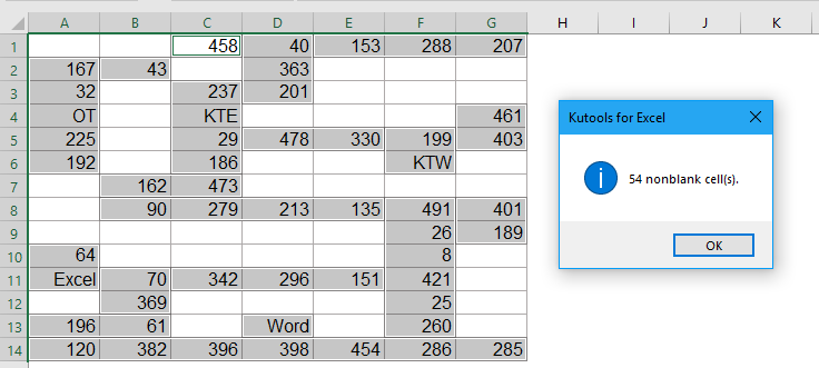
2. And then, all data cells will be selected at once, and a dialog box will pop out to remind you how many non blank cells are selected, see screenshot:

3. And then, you can fill the selected cells with font or background color as you need, see screenshot:

Click to Download Kutools for Excel and free trial Now!
More relative data validation articles:
- Highlight largest / lowest value in each row or column
- If you have multiple columns and rows data, how could you highlight the largest or lowest value in each row or column? It will be tedious if you identify the values one by one in each row or column. In this case, the Conditional Formatting feature in Excel can do you a favor. Please read more to know the details.
- Highlight Cells Based On Length Of Text In Excel
- Supposing you are working with a worksheet which has list of text strings, and now, you want to highlight all the cells that the length of the text is greater than 15. This artical, I will talk about some methods for solving this task in Excel.
- Highlight / Conditional Formatting Cells With Formulas In Excel
- Supposing you have a large worksheet which contains both constants and formulas, and now you want to know the location of all the formula cells. Of course, you can select all the formulas easily and quickly by using Go To Special function. But if your data or formulas need to be changed now and then, you must apply this function repeatedly.
- Highlight Duplicate Values In Different Colors In Excel
- In Excel, we can easily highlight the duplicate values in a column with one color by using the Conditional Formatting, but, sometimes, we need to highlight the duplicate values in different colors to recognize the duplicates quickly and easily as following screenshot shown. How could you solve this task in Excel?
- Highlight Rows Based On Drop Down List In Excel
- This article will talk about how to highlight rows based on drop down list, take the following screenshot for example, when I select “In Progress” from the drop down list in column E, I need to highlight this row with red color, when I select “Completed” from the drop down list, I need to highlight this row with blue color, and when I select “Not Started”, a green color will be used to highlight the row.
Best Office Productivity Tools
Supercharge Your Excel Skills with Kutools for Excel, and Experience Efficiency Like Never Before. Kutools for Excel Offers Over 300 Advanced Features to Boost Productivity and Save Time. Click Here to Get The Feature You Need The Most...
Office Tab Brings Tabbed interface to Office, and Make Your Work Much Easier
- Enable tabbed editing and reading in Word, Excel, PowerPoint, Publisher, Access, Visio and Project.
- Open and create multiple documents in new tabs of the same window, rather than in new windows.
- Increases your productivity by 50%, and reduces hundreds of mouse clicks for you every day!
All Kutools add-ins. One installer
Kutools for Office suite bundles add-ins for Excel, Word, Outlook & PowerPoint plus Office Tab Pro, which is ideal for teams working across Office apps.
- All-in-one suite — Excel, Word, Outlook & PowerPoint add-ins + Office Tab Pro
- One installer, one license — set up in minutes (MSI-ready)
- Works better together — streamlined productivity across Office apps
- 30-day full-featured trial — no registration, no credit card
- Best value — save vs buying individual add-in