Paste into Visible Cells Only: Skip Hidden Rows in Excel
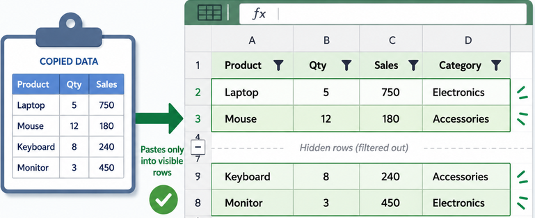
Excel has a well-known limitation that has frustrated users for years: when you copy data and try to paste it into a filtered (hidden rows) list, Excel often pastes into hidden rows as well, corrupting your data. This issue has cost users countless hours of rework and data recovery.
The core problem is that while Excel provides an easy way to copy only visible cells (using Alt+; or Go To Special), there is no built-in "Paste to Visible Cells Only" feature. When you paste into a filtered range, Excel pastes consecutively from the top-left cell of your selection, ignoring row visibility.
Below are several practical ways to paste or fill data into filtered rows only.
Paste the same value into visible cells only
Paste different values into visible cells only
- Method 1: With helper column
- Method 2: With VBA code
- Method 3: With Kutools for Excel (Quick and Easy)
Paste the same value into visible cells only
If you want to enter the same value into a filtered list, such as adding the same status, remark, or category to all visible rows, you don’t need to paste one by one. Excel allows you to select visible cells only, so the hidden rows will be skipped automatically.
This method is especially useful after applying a filter. For example, after filtering the Region column to show only East, you can fill the Status column with the same value, such as Completed, without affecting the rows that are hidden by the filter.
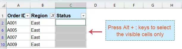
- Select the target cells in the filtered column.
- Press Alt + ; keys to select the visible cells only. See screenshot:
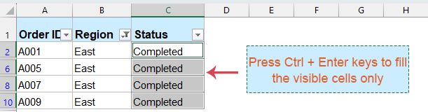
- Then, type the value you want to enter directly, and press Ctrl + Enter keys together, Excel fills only the visible cells, hidden rows are skipped.


Notes
- This method works well when all visible cells should receive the same value.
- If you need to paste a list of different values into visible rows, use the following methods.
Paste different values into visible cells only
If you need to paste a list of different values into a filtered table, things can be a little tricky. For example, after filtering the Region column to show only East, you may want to paste different status values such as Completed, Pending, Shipped, and Approved into the visible rows only. In this case, you need a safer method to make sure each value is pasted into the next visible cell, while all hidden rows remain unchanged.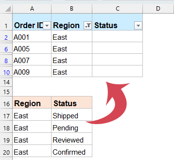
Method 1: With helper columns
If you need to paste a list of different values into a filtered list, normal copy and paste may not work correctly because filtered rows are not continuous. To avoid overwriting hidden rows, you can use two helper columns to temporarily sort and group the visible rows, paste the new data, and then restore the original order.
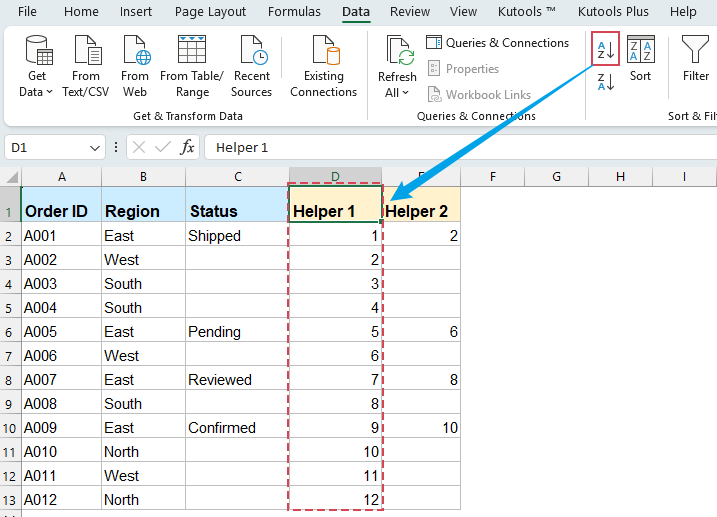
Step 1: Remove the filter and add an order helper column
- First, remove the existing filter by clicking Data > Filter.
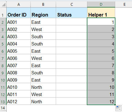
- Then add a helper column next to your data table to record the original row order. For example, enter 1 in cell D2 and 2 in cell D3, then select D2:D3 and drag the fill handle down to the last row of your data. This helper column will be used later to restore the original order after sorting and pasting. See screenshot:

Step 2: Filter the data and mark the visible rows
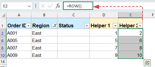
- Apply the filter again by clicking Data > Filter, and then filter the column based on your condition. For example, filter the data to show only East records.
- In another helper column, enter the following formula in the first visible row:
=ROW() - Then fill the formula down through the visible rows. This marks the filtered records so they can be grouped together in the next step.

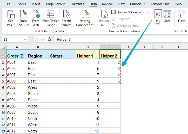
Step 3: Remove the filter and sort by the visible-row helper column
Remove the filter again. Then sort the table by the helper column that contains the ROW() results in ascending order. Now all filtered records will be grouped together as a continuous range.
Step 4: Paste the new data
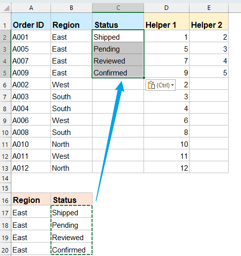
Copy the new data and paste it into the grouped records, because the target rows are now continuous, Excel can paste the data correctly without affecting the other records.
Step 5: Restore the original order
After pasting the new data, sort the table by the original order helper column in ascending order. This brings the worksheet back to its original row arrangement.
Step 6: Remove the helper columns
Finally, delete or clear the helper columns. You can apply the filter again to check the result. Only the records that matched the filter condition have been updated, while all other rows remain unchanged. See screenshot:

Note:
This method does not paste directly into non-adjacent visible cells. Instead, it temporarily groups the filtered rows together so that the new data can be pasted safely into a continuous range. After the data is pasted, the original row order is restored with the helper column.
Pros and Cons:
Pros:
- Works for different values
- Avoids overwriting hidden rows
- Suitable for older Excel versions
- Keeps the original order recoverable
Cons:
- More steps are required
- Easy to make mistakes if the helper columns are not set correctly
- Not ideal for very large datasets
- Temporarily changes the row order
Method 2: With VBA code
If you often need to paste different values into filtered rows, VBA is a more direct solution.
This macro takes values from a source range and pastes them into the visible cells of a filtered target range, skipping hidden rows.
- Hold down the ALT + F11 keys in Excel, and it opens the Microsoft Visual Basic for Applications window.
- Click Insert > Module, and paste the following code in the Module Window.
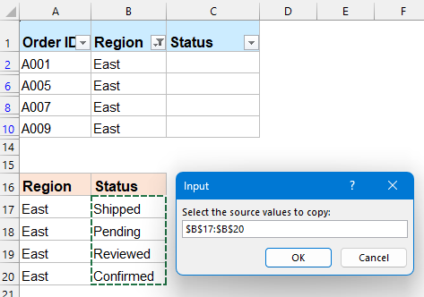
Sub PasteIntoVisibleCellsOnly() Dim SourceRange As Range Dim TargetRange As Range Dim VisibleCells As Range Dim Cell As Range Dim i As Long On Error Resume Next Set SourceRange = Application.InputBox("Select the source values to copy:", Type:=8) Set TargetRange = Application.InputBox("Select the filtered target range:", Type:=8) On Error GoTo 0 If SourceRange Is Nothing Or TargetRange Is Nothing Then Exit Sub On Error Resume Next Set VisibleCells = TargetRange.SpecialCells(xlCellTypeVisible) On Error GoTo 0 If VisibleCells Is Nothing Then MsgBox "No visible cells found in the target range.", vbExclamation Exit Sub End If If SourceRange.Cells.Count > VisibleCells.Cells.Count Then MsgBox "The source range contains more cells than the visible target range.", vbExclamation Exit Sub End If i = 1 For Each Cell In VisibleCells If i <= SourceRange.Cells.Count Then Cell.Value = SourceRange.Cells(i).Value i = i + 1 Else Exit For End If Next Cell MsgBox "Data has been pasted into visible cells only.", vbInformation End Sub - Press F5 key or click the Run button to run this code. A prompt box will appear, asking you to select the source values you want to copy. See screenshot:
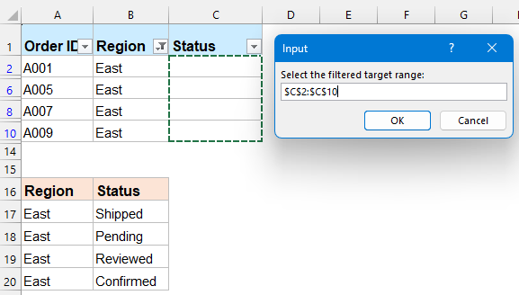
- Click OK, and in another box, select the filtered target range where you want to paste the data. See screenshot:
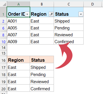
- Click OK, and the selected data will be pasted into visible rows only without affecting any hidden rows. See screenshot:


Pros:
- Works well for different values.
- Skips filtered-out rows automatically.
- Useful for repeated tasks.
Cons:
- Requires VBA.
- The workbook may need to be saved as .xlsm.
- Macros must be enabled.
Method 3: With Kutools for Excel
If you want a quicker and more beginner-friendly way to paste data into filtered rows only, Kutools for Excel can be a helpful option. Instead of using helper columns or VBA code, Kutools provides a more direct way to paste data into visible cells while automatically skipping hidden rows. It is a good choice for users who frequently work with filtered tables and want to avoid the risk of overwriting hidden data.
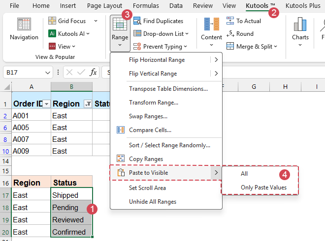
- Select the source data range that you want to copy and paste to the filtered list. And then click Kutools > Range > Paste to Visible > All / Only Paste Values, see screenshot:
Tip:
- If you choose Only Paste Values option, only values will be pasted into the filtered data;
- If you choose All option, the values as well as the formatting will be pasted into the filtered data.
- Then, a Paste to Visible Range prompt box is popped out, click a cell or a range cells where you want to paste the new data, see screenshot:
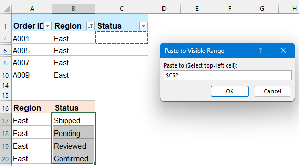
- And then click OK button, the new data has been pasted into the filtered list only, and the hidden rows data is kept as well.


Paste Data into Visible Rows Only with Kutools for Excel
When working with filtered data in Excel, normal copy and paste may affect hidden rows or fail with non-contiguous visible cells. Kutools for Excel provides a simple Paste to Visible feature that helps you paste data only into visible rows while automatically skipping hidden rows.
Skip Hidden Rows Automatically
Paste values only into visible rows after filtering, without overwriting hidden data.
Paste Different Values Easily
Quickly paste a list of different values into filtered rows in the correct order.
No Formulas or VBA
Avoid complex helper formulas, sorting steps, and macro code. Just select, paste, and finish.
Great for Filtered Tables
Ideal for updating statuses, remarks, categories, review results, or filtered records in bulk.
Important Notes When Pasting into Filtered Lists
- Normal paste may not work as expected
When a list is filtered, the visible rows are often non-adjacent. Excel may not paste copied data correctly into non-contiguous visible cells.
- Use Alt + ; carefully
Alt + ; selects visible cells only, but it is best for filling the same value or formula.
For a list of different values, VBA or a helper formula is safer.
- Always back up your data first
Before pasting into filtered data, make a copy of the worksheet. This helps avoid accidental overwriting.
- Check the source and target counts
When pasting different values, make sure the number of source values matches the number of visible target cells.
Conclusion
To paste data into a filtered list while skipping hidden rows, the best method depends on what you want to paste.
- For the same value, use Alt + ; and press Ctrl + Enter.
- For different values, use helper columns or VBA to safely match each value with visible rows only.
- If you prefer a visual and easier solution, Kutools for Excel can help you manage filtered and visible-cell operations more efficiently.
Best Office Productivity Tools
Supercharge Your Excel Skills with Kutools for Excel, and Experience Efficiency Like Never Before. Kutools for Excel Offers Over 300 Advanced Features to Boost Productivity and Save Time. Click Here to Get The Feature You Need The Most...
Office Tab Brings Tabbed interface to Office, and Make Your Work Much Easier
- Enable tabbed editing and reading in Word, Excel, PowerPoint, Publisher, Access, Visio and Project.
- Open and create multiple documents in new tabs of the same window, rather than in new windows.
- Increases your productivity by 50%, and reduces hundreds of mouse clicks for you every day!
All Kutools add-ins. One installer
Kutools for Office suite bundles add-ins for Excel, Word, Outlook & PowerPoint plus Office Tab Pro, which is ideal for teams working across Office apps.
- All-in-one suite — Excel, Word, Outlook & PowerPoint add-ins + Office Tab Pro
- One installer, one license — set up in minutes (MSI-ready)
- Works better together — streamlined productivity across Office apps
- 30-day full-featured trial — no registration, no credit card
- Best value — save vs buying individual add-in
Table of contents
- Paste the same value into visible cells only
- Paste different values into visible cells only
- Method 1: With helper column
- Method 2: With VBA code
- Method 3: With Kutools for Excel (Quick and Easy)
- Important Notes When Pasting into Filtered Lists
- Conclusion
- The Best Office Productivity Tools
Kutools for Excel
Brings 300+ advanced features to Excel
- ⬇️ Free Download
- 🛒 Purchase Now
- 📘 Feature Tutorials
- 🎁 30-Day Free Trial