The ultimate guide to searchable drop-down list in Excel
Creating drop-down lists in Excel streamlines data entry and minimizes errors. But with larger datasets, scrolling through lengthy lists becomes cumbersome. Wouldn't it be easier to just type and quickly locate your item? A "searchable drop-down list" offers this convenience. This guide will walk you through four methods to set up such a list in Excel.

- Searchable drop-down list in Excel 365
- Create searchable drop-down list (for Excel 2019 and later)
- Create searchable drop-down list easily (for all Excel versions)
- Create searchable drop-down list with Combo box and VBA (more complex)
Searchable drop-down list in Excel 365
Excel 365 has introduced a much-anticipated feature to its data validation drop-down lists: the ability to search within the list. With the searchable functionality, users can quickly locate and select items in a more efficient manner. After inserting the drop-down list as usual, just click on a cell with a drop-down list and start typing. The list will instantly filter to match the typed text.
In this case, I type San in the cell and the drop-down list filters out cities that start with the search term San, such as San Francisco and San Diego. Then you can select a result with your mouse or use the arrow keys and press Enter.

- The search is initiated from the first letter of each word in the drop-down list. If you input a character that doesn't match the starting character of any word, the list won't display matching items.
- This feature is only available in the latest version of Excel 365.
- If your version of Excel does not support this feature, here we recommend the Searchable Drop-down List feature of Kutools for Excel. There is no Excel version limitation, and once enabled, you can easily search for the desired item in the drop-down list by simply typing the relevant text. View the detailed steps.
Create searchable drop-down list (for Excel 2019 and later)
If you are using Excel 2019 or later versions, the method in this section can also be used to make a drop-down list searchable in Excel.
Assuming you have created a drop-down list in cell A2 of Sheet2 (image on the right) using data in the range A2:A8 of Sheet1 (image on the left), follow these steps to make the list searchable.

Step 1. Create a helper column that lists the search items
Here we need a helper column to list the items that matching your source data. In this case, I will create the helper column in column D of Sheet1.
- Select the first cell D1 in column D and enter the column header, such as "Search results" in this case.
- Enter the following formula into cell D2 and press Enter.
=FILTER(A2:A8,ISNUMBER(SEARCH(Sheet2!A2,A2:A8)),"Not Found")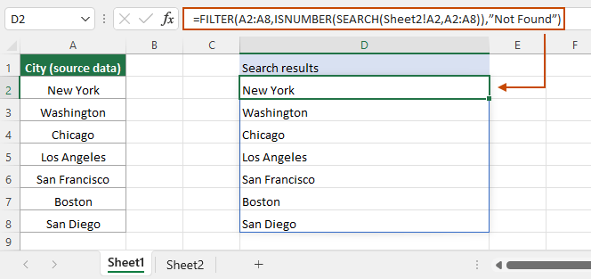
- In this formula, A2:A8 is the source data range. Sheet2!A2 is the location of the drop-down list, which means the drop-down list is located in A2 of Sheet2. Please change them according to your own data.
- If no item is selected from the drop-down list in A2 of Sheet2, the formula will display all items from the source data, as depicted in the image above. Conversely, if an item is selected, D2 will display that item as the result of the formula.
Step 2: Reconfigure the drop-down list
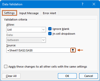
- Select the drop-down list cell (in this case, I select the cell A2 of Sheet2), then go to select Data > Data Validation > Data Validation.

- In the Data Validation dialog box, you need to configure as follow.
- Under the Settings tab, click the
 button in the Source box.

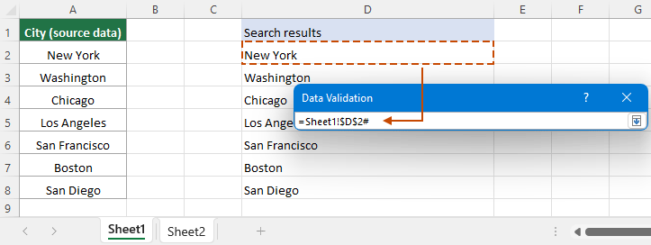
- The Data Validation dialog box will redirect to Sheet1, select the cell (e.g., D2) with the formula from Step 1, add a # symbol, and click the Close button.

- Go to the Error Alert tab, uncheck the Show error alert after invalid data is entered checkbox, and finally click the OK button to save the changes.

- Under the Settings tab, click the
Result
The drop-down list in cell A2 of Sheet2 is now searchable. Type text in the cell, click the drop-down arrow to expand the drop-down list, and you will see the list instantly filtered to match the typed text.

- This method is only available for Excel 2019 and later versions.
- This method only works on one drop-down list cell at a time. To make drop-down lists searchable in cells A3 through A8 in Sheet2, the aforementioned steps must be repeated for each cell.
- When you type text in the drop-down list cell, the drop-down list does not expand automatically, you need to click the drop-down arrow to expand it manually.
Create searchable drop-down list easily (for all Excel versions)
Given the various limitations of the above methods, here is a very effective tool for you - Kutools for Excel's Make Drop-down List Searchable, Auto-popupfeature. This feature is available in all versions of Excel and allows you to easily search for the desired item in the drop-down list with a simple setup.
After downloading and installing Kutools for Excel, select Kutools > Drop-down List > Make Drop-down List Searchable, Auto-popup to enable this feature. In the Make the Drop-down List Searchable dialog box, you need to:
- Select the range containing the drop-down lists that need to be set as searchable drop-down lists.
- Click OK to complete the settings.
Result
When you click a drop-down list cell in the specified range, a list box appears to the right. Type text to filter the list instantly, then select an item or use arrow keys and hit Enter to add it to the cell.
- This feature supports searching from any position within the words. This means even if you input a character that's in the middle or end of a word, matching items will still be found and displayed, offering a more comprehensive and user-friendly search experience.
- To know more about this feature, please visit this page.
- To apply this feature, please download and install Kutools for Excel first.
Create searchable drop-down list with Combo box and VBA (more complex)
If you simply want to create a searchable drop-down list without specifying a particular drop-down list type. This section provides an alternative approach: using a Combo box with VBA code to achieve the task.
Suppose you have a list of country names in column A as shown in the screenshot below, and now you want to use them as the source data of the searchale drop-down lists, you can do as follows to get it done.

You need to insert a Combo box instead of a data validation drop-down list in your worksheet.
- If the Developer tab does not display on the ribbon, you can enable the Developer tab as follows.
- In Excel 2010 or later versions, click File > Options. And in the Excel Options dialog box, click Customize Ribbon in the left pane. Go to the Customize the Ribbon list box, check the Developer box, and then click the OK button. See screenshot:

- In Excel 2007, click Office button > Excel Options. In the Excel Options dialog box, click Popular in the left pane, check the Show Developer tab in the Ribbon box, and finally click the OK button.

- In Excel 2010 or later versions, click File > Options. And in the Excel Options dialog box, click Customize Ribbon in the left pane. Go to the Customize the Ribbon list box, check the Developer box, and then click the OK button. See screenshot:
- After showing the Developer tab, click Developer > Insert > Combo box.

- Draw a Combo box in the worksheet, right click it and then select Properties from the right-clicking menu.

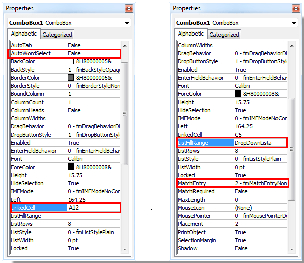
- In the Properties dialog box, you need to:
- Select False in the AutoWordSelect field;
- Specify a cell in the LinkedCell field. In this case, we enter A12;
- Select 2-fmMatchEntryNone in the MatchEntry field;
- Type DropDownList into the ListFillRange field;
- Close the Properties dialog box. See screenshot:

- Now turn off the design mode by clicking Developer > Design Mode.
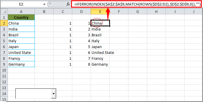
- Select a blank cell such as C2, enter the formula below and press Enter. They drag its AutoFill Handle down to cell C9 to auto fill the cells with the same formula. See screenshot:
=--ISNUMBER(IFERROR(SEARCH($A$12,A2,1),"")) Notes:
- $A$12 is the cell that you have specified it as the LinkedCell in step 4;
- After finishing the above steps, you can now test: enter a letter C in the combo box, and then you can see that the formula cells that reference the cells containing the character C are filled with the number 1.
- Select the cell D2, enter the formula below and press Enter. Then drag its AutoFill Handle down to the cell D9.
=IF(C2=1,COUNTIF($C$2:C2,1),"")
- Select cell E2, enter the formula below and press Enter. Then drag its AutoFill Handle down to E9 to apply the same formula.
=IFERROR(INDEX($A$2:$A$9,MATCH(ROWS($D$2:D2),$D$2:$D$9,0)),"")
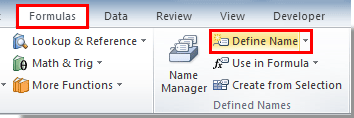
- Now you need to create a name range. Please click Formula > Define Name.

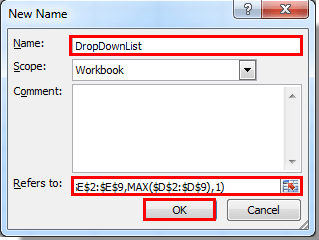
- In the New Name dialog box, type DropDownList in the Name box, enter the formula below in the Refers to box, and then click the OK button.
=$E$2:INDEX($E$2:$E$9,MAX($D$2:$D$9),1)
- Now, turn on the design mode by clicking Developer > Design Mode. Then double click the Combo box to open the Microsoft Visual Basic for Applications window.
- Copy and paste the VBA code below into the Code editor.
 VBA code: make drop down list searchable
Private Sub ComboBox1_GotFocus() ComboBox1.ListFillRange = "DropDownList" Me.ComboBox1.DropDown End Sub - Press the Alt + Q keys to close the Microsoft Visual Basic for Applications window.
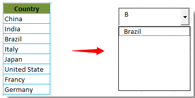
From now on, when a character is entered in the combo box, it will do a fuzzy search and then list the relevant values in the list.
Related articles:
Autocomplete when typing in Excel drop down list
If you have a data validation drop down list with large values, you need to scroll down in the list just for finding the proper one, or type the whole word into the list box directly. If there is method for allowing to auto complete when typing the first letter in the drop down list, everything will become easier. This tutorial provides the method to solve the problem.
Create drop down list from another workbook in Excel
It is quite easy to create a data validation drop down list among worksheets within a workbook. But if the list data you need for the data validation locates in another workbook, what would you do? In this tutorial, you will learn how to create a drop fown list from another workbook in Excel in details.
Create a searchable drop down list in Excel
For a drop down list with numerous values, finding a proper one is not an easy work. Previously we have introduced a method of auto completing drop down list when enter the first letter into the drop down box. Besides the autocomplete function, you can also make the drop down list searchable for enhancing the working efficiency in finding proper values in the drop down list. For making drop down list searchable, try the method in this tutorial.
Auto populate other cells when selecting values in Excel drop down list
Let’s say you have created a drop down list based on the values in cell range B8:B14. When you selecting any value in the drop down list, you want the corresponding values in cell range C8:C14 be automatically populated in a selected cell. For solving the problem, the methods in this tutorial will do you a favor.
The Best Office Productivity Tools
Kutools for Excel - Helps You To Stand Out From Crowd
Kutools for Excel Boasts Over 300 Features, Ensuring That What You Need is Just A Click Away...
Office Tab - Enable Tabbed Reading and Editing in Microsoft Office (include Excel)
- One second to switch between dozens of open documents!
- Reduce hundreds of mouse clicks for you every day, say goodbye to mouse hand.
- Increases your productivity by 50% when viewing and editing multiple documents.
- Brings Efficient Tabs to Office (include Excel), Just Like Chrome, Edge and Firefox.
Table of contents
Create searchable drop-down list
- Video
- For Excel 365
- For Excel 2019 and later versions
- For all Excel versions (easily)
- For all Excel versions (complex VBA)
- Related Articles
- The Best Office Productivity Tools
- Comments


 button in the Source box.
