
How to extract unique values based on criteria in Excel?

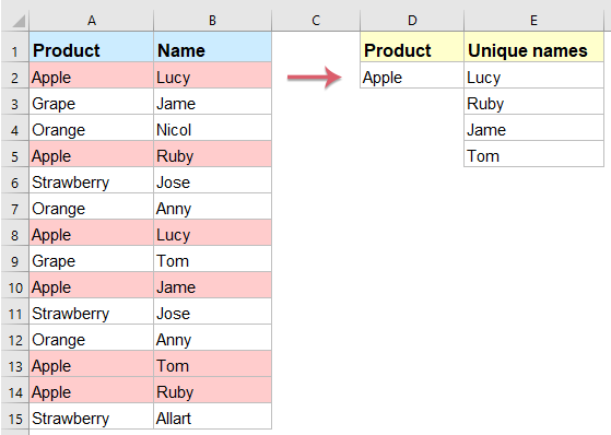
Supposing, you have the left data range that you want to list only the unique names of column B based on a specific criterion of column A to get the result as below screenshot shown. How could you deal with this task in Excel quickly and easily?

Extract unique values based on criteria with array formula

Extract unique values based on multiple criteria with array formula

Extract unique values from a list of cells with a useful feature


Extract unique values based on criteria with array formula

To solve this job, you can apply a complex array formula, please do as follows:

1. Enter the below formula into a blank cell where you want to list the extracting result, in this example, I will put it to cell E2, and then press Shift + Ctrl + Enter keys to get the first unique value.

=IFERROR(INDEX($B$2:$B$15, MATCH(0, IF($D$2=$A$2:$A$15, COUNTIF($E$1:$E1, $B$2:$B$15), ""), 0)),"")

2. Then, drag the fill handle down to the cells until blank cells are displayed, and now all the unique values based on the specific criterion have been listed, see screenshot:

Note: In the above formula: B2:B15 is the column range contains the unique values that you want to extract from, A2:A15 is the column contains the criterion you based on, D2 indicates the criterion that you want to list the unique values based on, and E1 is the cell above your entered formula.

Extract unique values based on multiple criteria with array formula

If you want to extract the unique values based on two conditions, here is another array formula can do you a favor, please do as this:

1. Enter the below formula into a blank cell where you want to list the unique values, in this example, I will put it to cell G2, and then press Shift + Ctrl + Enter keys to get the first unique value.

=IFERROR(INDEX($C$2:$C$15,MATCH(0,COUNTIF(G1:$G$1,$C$2:$C$15)+IF($A$2:$A$15<>$E$2,1,0)+IF($B$2:$B$15<>$F$2,1,0),0)),"")

2. Then, drag the fill handle down to the cells until blank cells are displayed, and now all the unique values based on the specific two conditions have been listed, see screenshot:

Note: In the above formula: C2:C15 is the column range contains the unique values that you want to extract from, A2:A15 and E2 are the first range with the criteria that you want to extract unique values based on, B2:B15 and F2 are the second range with the criteria that you want to extract unique values based on, and G1 is the cell above your entered formula.

Extract unique values from a list of cells with a useful feature

Sometimes, you just want to extract the unique values from a list of cells, here, I will recommend a useful tool-Kutools for Excel, with its Extract cells with unique values (include the first duplicate) utility, you can quickly extract the unique values.

Note:To apply this Extract cells with unique values (include the first duplicate), firstly, you should download the Kutools for Excel, and then apply the feature quickly and easily.

After installing Kutools for Excel, please do as this:

1. Click a cell where you want to output the result. (Note:Don't click a cell in the first row.)

2. Then click Kutools > Formula Helper > Formula Helper, see screenshot:

3. In the Formulas Helper dialog box, please do the following operations:

  • Select Text option from the Formula Type drop down list;
  • Then choose Extract cells with unique values (include the first duplicate) from the Choose a fromula list box;
  • In the right Arguments input section, select a list of cells that you want to extract unique values.

4. Then click Ok button, the first result is displayed into the cell, then select the cell and drag the fill handle over to the cells that you want to list all the unique values until blank cells are shown, see screenshot:

Free Download Kutools for Excel Now!


More relative articles:

  • Count The Number Of Unique And Distinct Values From A List
  • Supposing, you have a long list of values with some duplicate items, now, you want to count the number of unique values (the values that appear in the list only once ) or distinct values (all different values in the list, it means unique values +1st duplicate values) in a column as left screenshot shown. This article, I will talk about how to deal with this job in Excel.
  • Sum Unique Values Based On Criteria In Excel
  • For example, I have a range of data which contains Name and Order columns, now, to sum only unique values in Order column based on the Name column as following screenshot shown. How to solve this task quickly and easily In Excel?
  • Concatenate Unique Values In Excel
  • If I have a long list of values which populated with some duplicate data, now, I want to find only the unique values and then concatenate them into a single cell. How could I deal with this problem quickly and easily in Excel?

Best Office Productivity Tools

Supercharge Your Spreadsheets: Experience Efficiency Like Never Before with Kutools for Excel

Popular Features: Find/Highlight/Identify Duplicates   |  Delete Blank Rows   |  Combine Columns or Cells without Losing Data   |   Round without Formula ...
Super Lookup: Multiple Criteria VLookup    Multiple Value VLookup  |   VLookup Across Multiple Sheets   |   Fuzzy Lookup ....
Advanced Drop-down List: Quickly Create Drop Down List   |  Dependent Drop Down List   |  Multi-select Drop Down List ....
Column Manager: Add a Specific Number of Columns     Move Columns   |   Unhide Columns   |   Compare Columns to Select Same & Different Cells ...
Featured Features: Grid Focus   |  Design View   |   Big Formula Bar    Workbook & Sheet Manager   |  Resource Library (Auto Text)   |  Date Picker   |  Combine Worksheets   |  Encrypt/Decrypt Cells    Send Emails by List   |  Super Filter   |   Special Filter (filter bold/italic/strikethrough...) ...
Top 15 Toolset12 Text Tools (Add Text, Remove Characters, ...)   |   50+ Chart Types (Gantt Chart, ...)   |   40+ Practical Formulas (Calculate age based on birthday, ...)   |   19 Insertion Tools (Insert QR Code, Insert Picture from Path, ...)   |   12 Conversion Tools (Numbers to Words, Currency Conversion, ...)   |   7 Merge & Split Tools (Advanced Combine Rows, Split Cells, ...)   |   Many More...

Kutools for Excel boasts over 300 features, ensuring that what you need is just a click away...

Supports Office/Excel 2007-2021 & newer, including 365   |   Available in 44 languages   |   Enjoy a full-featured 30-day free trial.

kte tab 201905


Office Tab Brings Tabbed interface to Office, and Make Your Work Much Easier

  • Enable tabbed editing and reading in Word, Excel, PowerPoint, Publisher, Access, Visio and Project.
  • Open and create multiple documents in new tabs of the same window, rather than in new windows.
  • Increases your productivity by 50%, and reduces hundreds of mouse clicks for you every day!
Comments (40)
No ratings yet. Be the first to rate!
This comment was minimized by the moderator on the site
Thank you so much. This was very very helpful. You Rock!!
This comment was minimized by the moderator on the site
hi everyone..
i have problem..
i got blank result even i press ctrl shift enter together..
This comment was minimized by the moderator on the site
Hi all, Can some help me to get all unique values on one single cell
This comment was minimized by the moderator on the site
Hi, this worked well! Although it takes Excel sooooo long to calculate. Just dragging down 15 cells in a column takes about 15min to calculate... if not longer. Is this normal? If this becomes dynamic it will take a hell of alot of computing time.
This comment was minimized by the moderator on the site
Hello. This is really helpful, however, what If I want a formula that lists the unique values based on multiple criteria. eg. I have a data set which has the following data in a table (after each hyphen is a new column but same row):

Company A - £200 - £100
Company A - £300 - £200
Company B - £300 - £200
Company C - £600 - £200
Company B - £100 - £300
Company D - £0 - £600
Company A - £700 - £100

I want a new data table in a new tab which groups the duplicate values without using an array formula. currently I'm grouping using a pivot table and pasting to my new data table. It's a long process but array formulas make my spreadsheet really slow.

Company A - £1200 - £400
Company B - £400 - £500
Company C - £600 - £200
Company D - £0 - £600

Thanks,
K
This comment was minimized by the moderator on the site
Hello, K,
For solving your problem, I can recommend our useful tool- Kutools for Excel, with its Advanced Combine Rows feature, you can deal with this job quickly. Firstly, you should copy and paste your data into a new worksheet, and then apply htis feature as below screenhsot shown.
You can know more about this feature from: https://www.extendoffice.com/product/kutools-for-excel/excel-combine-duplicate-rows.html
Please download Kutools for Excel and install it, then apply this feature. Full feature free trial 30-day, please try.
This comment was minimized by the moderator on the site
Hi! the formula works really well. I would like to add another criterion, i mean, get the unique answers but using two criteria
This comment was minimized by the moderator on the site
Hi, Giancarlo,
to extract unique values based on multiple criteria, any of the below formula can help you: (after pasting the formula, please press Ctrl + Shift + Enter keys together.)
=IFERROR(INDEX($C$2:$C$11, MATCH(0, COUNTIF(G1:$G$1, $C$2:$C$11)+IF($A$2:$A$11<>$E$2, 1, 0)+IF($B$2:$B$11<>$F$2, 1, 0), 0)), "")
=INDEX($C$2:$C$11, MATCH(0, IF(($A$2:$A$11=$E$2)*($B$2:$B$11=$F$2), COUNTIF($G$1:$G1, $C$2:$C$11), ""), 0))
Please try, hope it can help you!
This comment was minimized by the moderator on the site
Hi. I am using the two conditions formula =IFERROR(INDEX($C$2:$C$11, MATCH(0, COUNTIF(G1:$G$1, $C$2:$C$11)+IF($A$2:$A$11<>$E$2, 1, 0)+IF($B$2:$B$11<>$F$2, 1, 0), 0)), "") to extract a unique list and it works great, but I am struggle to add the SMALL function to get the list sorted as well in ascending order. Are you able to help?
This comment was minimized by the moderator on the site
Is there a way to make this work while ALLOWING for duplicate values? For instance, I want all instances of Lucy to be listed in the results.
This comment was minimized by the moderator on the site
Hello, Konstantin,
To extract all corresponding values including the duplicates based on a specific cell criteria, the following array formula can help you, see screenshot:
=IF(ISERROR(INDEX($A$1:$B$17,SMALL(IF($A$1:$A$17=$D$2,ROW($A$1:$A$17)),ROW(1:1)),2)),"",
INDEX($A$1:$B$17,SMALL(IF($A$1:$A$17=$D$2,ROW($A$1:$A$17)),ROW(1:1)),2))

After inserting the formula, please press Shift + Ctrl + Enter keys together to get the correct result, and then drag the fill handle down to get all values.
Hope this can help you, thank you!
This comment was minimized by the moderator on the site
This has worked great for me with a specific lookup value. However, if I wanted to use a wildcard to look up partial values, how would I do that? For example, if I wanted to lookup all the names associated with KT?

I am using this function to look up cells that contain multiple text. For example if each product also had a sub-product within the same cell but I was only looking for names associated with the sub-product "elf".

KTE - elf
KTE- ball
KTE - piano
KTO - elf
KTO- ball
KTO - piano
This comment was minimized by the moderator on the site
For me the formula does not work. I press ctrl shift enter and i still get an error N/A. I would like to add that i prpared exaclty the same data as in tutorial. What is the reason it does not work?
This comment was minimized by the moderator on the site
How would I get this formula to return each of the duplicates instead of one of each of the names? For instance, in the example above, how would I get the results column (B:B) to return Lucy, Ruby, Anny, Jose, Lucy, Anny, Tom? I'm using this as a budget tool pulling to specific account summaries from a general ledger. However, several of the amounts and transaction descriptions are duplicates in the general ledger. Once the first of the duplicated values is pulled, no more of them get pulled.
This comment was minimized by the moderator on the site
Hi, Joe,
To extract all corresponding values based on a specific cell criteria, the following array formula can help you, see screenshot:
=IF(ISERROR(INDEX($A$1:$B$17,SMALL(IF($A$1:$A$17=$D$2,ROW($A$1:$A$17)),ROW(1:1)),2)),"",
INDEX($A$1:$B$17,SMALL(IF($A$1:$A$17=$D$2,ROW($A$1:$A$17)),ROW(1:1)),2))

After inserting the formula, please press Shift + Ctrl + Enter keys together to get the correct result, and then drag the fill handle down to get all values.
Hope this can help you, thank you!
This comment was minimized by the moderator on the site
Last Question: If I want the results column to return all values not associated with KTE or KTO (so, D:D would be Tom, Nocol, Lily, Angelina, Genna), how would I do that?
This comment was minimized by the moderator on the site
Ok, so it works in the master workbook. There is one exception that I haven't been able to determine the cause of: If the array (in my case, the general ledger that I had beginning in row 3) does not begin in Row 1, the returned values are incorrect. What causes this problem, and which term in the formula fixes it? Thanks again for your help with this!
This comment was minimized by the moderator on the site
So far so good. I'm able to duplicate the results in the test sheet, make changes to the array, and then correct the formula to account for the changes I've made. I plan to move this into the master sheet today and see how it works. Thanks for the help!
This comment was minimized by the moderator on the site
Thank You!
This comment was minimized by the moderator on the site
I am getting 0 instead of the expected results, the formula is doing great for data in the same sheet, do you have any solution for data in different sheet ?

this is my formula

=IFERROR(INDEX('Switching Data'!$B$7:$B$204,MATCH(0,IF($A$2='Switching Data'!$A$7:$A$204,COUNTIF($A$4:A4,'Switching Data'!$B$7:$B$204),""),0)),0)
This comment was minimized by the moderator on the site
Hello Gon, I hope you are well. I wonder if you can to resolve this issue. I am getting same error when formula come from different sheet. I will appreciate share the solution if you got it.
This comment was minimized by the moderator on the site
Hi, Gon,
After inserting the formula, you should press Ctrl + Shift + Enter keys together, not just Enter key.
Please try it, thank you!
This comment was minimized by the moderator on the site
If you get the #N/A error, go to your formula and use Control + Shift + Enter instead of Enter.
This comment was minimized by the moderator on the site
Hello, I am getting "#N/A" error at "Match function", can you please guide?
This comment was minimized by the moderator on the site
I am getting #N/A error at Match function with this formula.Can you please help?
This comment was minimized by the moderator on the site
actually I want the cell to reflect "YES" if (AL2="AP" and AK2="AD" and Z2>500000)
This comment was minimized by the moderator on the site
=IF(AL2="AP","AP",IF(AK2="AD","AD",IF(Z2>500000,"Yes","No"))) I want "all conditions" to be satisfied to say yes...excel reflecting error in this formula..pls advise
This comment was minimized by the moderator on the site
this was super helpful, but I keep getting doubles of all the names like this:
Doe, Jane
Doe, Jane
Hoover, Tom
Hoover, Tom

How can I stop this?
This comment was minimized by the moderator on the site
Hello, I am getting "#N/A" error at "Match function", can you please guide?
This comment was minimized by the moderator on the site
Hi Ryan. Formulas works great, however when dragging down the first value keeps repeating. I have made sure that COUNTIF references the cell ABOVE the cell with the formula, but still repeats the first value when dragging down? (eg. if the array formula is in C2 then COUNTIF points to cell $C$1:$C$1)
This comment was minimized by the moderator on the site
Probably doesn`t work cause you´ve locked the cells - Try to replace $C$1:$C$1 with $C$1:$C1
This comment was minimized by the moderator on the site
Hi, to stop the first value repeating as you drag down you must COUNTIF the cell ABOVE the cell you're putting the formula in. E.g if the formula is going in E2 you must type countif($E$1:$E1...
This comment was minimized by the moderator on the site
Hi Ryan. Formulas works great, however when dragging down the first value keeps repeating. I have made sure that COUNTIF references the cell ABOVE the cell with the formula, but still repeats the first value when dragging down? (eg. if the array formula is in C2 then COUNTIF points to cell $C$1:$C$1)
This comment was minimized by the moderator on the site
When using this formula it keeps repeating the first value, how do you make that stop and provide the list of values that equals the product in D2?
This comment was minimized by the moderator on the site
This works really well, but whenever the value that it is putting in is duplicated, it only places the value once. For example, if your list had two Lucy's in it, it only brings one Lucy over to the new table. Is there a way to fix this?
This comment was minimized by the moderator on the site
Thanks for this I have tried this and seems to be working fine intermittently. The issue that keeps repeating is that sometimes only the first matched value will return and is then duplicated when I am dragging down to return all matched values. How do I prevent this? Any suggestions?
This comment was minimized by the moderator on the site
Thank You, This is great!
This comment was minimized by the moderator on the site
Thank you for this tutorial! I'm also trying to modify the formula, like the above commentator, but with an AND condition so it meets another conditional criteria (e.g. for this example, I'd like to see only things above a certain threshold). Can you please advise? Thank you!
This comment was minimized by the moderator on the site
Hey, One way to do it: Replace the if formula with sumproduct((condition1=rng1)+(condition2=rng2))*countif(... It worked for me. Good luck! By replacing the + with an * you can make it an OR condition, but take good care of the brackets!
This comment was minimized by the moderator on the site
Hi, thanks for this tutorial, it works perfectly. I'm trying to modify it to work with an OR condition, but it doesn't seem to be working - is this possible? e.g. =INDEX($B$2:$B$17, MATCH(0, IF(OR($D$2=$A$2:$A$17,$D$2=$B$2:$B$17), COUNTIF($E$1:$E1, $B$2:$B$17), ""), 0))
There are no comments posted here yet
Please leave your comments in English
Posting as Guest
×
Rate this post:
0   Characters
Suggested Locations