How to calculate the correlation coefficient between two variables in Excel?
We usually use the correlation coefficient (a value ranging from -1 to1) to indicate the strength and direction of the linear relationship between two variables. A correlation coefficient is a widely used statistic that helps you understand relationships such as the connection between sales and advertising spend, temperature and ice cream sales, or other paired data. In Excel, there are multiple straightforward methods for calculating the correlation coefficient, including built-in functions and analysis tools.
Method A: Directly use CORREL function
Method B: Apply Data Analysis and output the analysis
Method C: Use PEARSON function as an alternative
Method D: Use VBA code to calculate correlation coefficients for multiple pairs
Method A: Directly use CORREL function
Consider two lists of data, each representing a variable. If you want to calculate the correlation coefficient between these two variables in Excel, this method is both quick and efficient.
For practical usage, ensure that both data ranges are numeric and contain the same number of observations. For example, if you have the following paired data:
Select a blank cell where you wish to display the calculation result. Enter the following formula, and then press the "Enter" key to calculate the correlation coefficient:
=CORREL(A2:A7,B2:B7)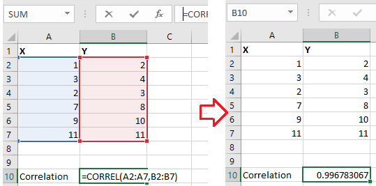
In this formula, A2:A7 and B2:B7 represent the two lists of variables you want to analyze. The ranges must be of equal length, and each pair should correspond to the same observation.
Practical tip: CORREL automatically ignores empty cells and text, but if there are no valid numeric pairs in the two columns, it will return a #DIV/0! error. Ensure your data is properly aligned and contains numeric pairs for an accurate correlation calculation.
Once you've calculated the correlation coefficient, you can insert a line chart to observe the relationships visually and further interpret the correlation, as shown below:
This method is best for quick, manual checks between two small data sets or when working interactively within your spreadsheet. It’s well-suited for users seeking an immediate result without the need for advanced statistical output.

Unlock Excel Magic with Kutools AI
- Smart Execution: Perform cell operations, analyze data, and create charts—all driven by simple commands.
- Custom Formulas: Generate tailored formulas to streamline your workflows.
- VBA Coding: Write and implement VBA code effortlessly.
- Formula Interpretation: Understand complex formulas with ease.
- Text Translation: Break language barriers within your spreadsheets.
Method B: Apply Data Analysis and output the analysis
If you need to analyze correlation between multiple variables at once or want a more comprehensive output table, Excel’s “Analysis Toolpak” provides a useful solution. This add-in generates a correlation matrix and allows you to compare several variables in a single step, which is valuable for larger datasets or building statistical reports.
1. If you have already added the Data Analysis add-in to your Data tab, you can skip to step3. Otherwise, click File > Options. In the “Excel Options” dialog, choose Add-Ins from the left pane, and then click the Go button next to the “Excel Add-ins” box.
2. In the “Add-Ins” dialog, check the box labeled Analysis ToolPak, then click OK. This will add the "Data Analysis" group to the Data tab.
3. Next, click Data > Data Analysis. In the pop-up “Data Analysis” dialog, choose Correlation from the list and then click OK.

4. In the Correlation dialog box, configure the following:
1) Select the range containing your data.
2) Choose either the "Columns" or "Rows" option, depending on how your data is organized.
3) If your data includes headers, check the “Labels in first row” option.
4) Specify an output location in “Output options” to display the results.
5. Click OK to generate the correlation analysis table. The correlation coefficients will be presented in the specified range.
This method is suitable when you need to evaluate the relationships among more than two variables or desire a summary table for reporting purposes. Data Analysis output is concise but does not provide additional significance statistics. If you receive unexpected results, double-check your data for consistency, empty cells, and correct range selection.
Method C: Use PEARSON function as an alternative
Besides CORREL, Excel provides the PEARSON function, which also calculates the Pearson correlation coefficient between two variables. Functionally, PEARSON and CORREL return the same result. However, PEARSON adheres strictly to the original mathematical formula, while CORREL is optimized for Excel’s environment. If you’re used to statistical theory or working with statistical tools outside Excel, PEARSON might feel more familiar.
For example, with two numeric lists in A2:A7 and B2:B7, you can calculate the correlation as follows:
1. Select a cell where you want to display the result, and enter this formula:
=PEARSON(A2:A7,B2:B7)2. Press Enter to complete the calculation. If you wish to analyze additional pairs of data, adjust the cell ranges accordingly, or drag the formula to other cells.
Tips: PEARSON ignores text or logical values, so ensure both ranges contain solely numeric values and are of equal length. If there is missing data in one column, align your ranges accordingly to avoid errors.
Using PEARSON is especially practical for users migrating from other statistical software, or for academic settings where strict adherence to terminology is expected. Both CORREL and PEARSON give the same result for typical use cases in Excel.
If you encounter a #DIV/0! error, check that both ranges are equal in length and contain no unmatched empty or non-numeric cells.
Pros: Easy to use, consistent with statistical software; Cons: Offers no significant difference from CORREL for most users.
Method D: Use VBA code to calculate correlation coefficients for multiple pairs
If you need to automate the calculation of correlation coefficients for several pairs of data (for instance, when working with many variable combinations), writing a simple VBA macro is an efficient choice. This method is well suited to advanced users who want to process large datasets or automate repetitive analysis tasks.
1. To use this method, first open the VBA editor by clicking Developer > Visual Basic. In the Visual Basic for Applications window, go to Insert > Module, and then paste the following code into the module:
Sub BatchCalculateCorrelations()
    Dim ws As Worksheet
    Dim rng1 As Range, rng2 As Range
    Dim lastRow As Long
    Dim i As Long
    Dim resultCol As Range

    On Error Resume Next
    xTitleId = "KutoolsforExcel"

    Set ws = ActiveSheet
    Set rng1 = Application.InputBox("Select first variable range (single column)", xTitleId, Type:=8)
    Set rng2 = Application.InputBox("Select second variable range (multiple columns)", xTitleId, Type:=8)
    Set resultCol = Application.InputBox("Select starting cell for output", xTitleId, Type:=8)

    If rng1.Rows.Count <> rng2.Rows.Count Then
        MsgBox "The two data ranges must have the same number of rows.", vbCritical, xTitleId
        Exit Sub
    End If

    For i = 1 To rng2.Columns.Count
        resultCol.Cells(1, i).Value = "Correlation with " & rng2.Cells(1, i).EntireColumn.Column
        resultCol.Cells(2, i).Value = WorksheetFunction.Correl(rng1, rng2.Columns(i))
    Next i
End Sub2. After inserting the code, close the VBA editor. In Excel, press Alt + F8, select BatchCalculateCorrelations, and click Run. You will be prompted to select:
- The first variable range (a single column, e.g. A2:A7)
- The second variable range (one or more columns, e.g. B2:D7)
- The cell where you want the results to start (e.g. F2)
The macro then calculates the correlation coefficient between the first variable and each column in the second range, displaying results horizontally from the chosen cell.
Advantages: Automates repetitive calculations, saves significant time with large datasets, and ensures consistency.
If you encounter issues such as “The two data ranges must have the same number of rows”, ensure all selected columns share the exact same row count and have no blank rows. For error troubleshooting, verify whether macros are enabled and ranges are selected correctly.
When working with correlation coefficients in Excel, choosing the right method depends on your data structure and analysis needs. For one-time, quick calculations between two series, formulas like CORREL or PEARSON are efficient and easy to use. For multiple variables or the need for summary tables, the Analysis Toolpak is very practical. If you require repeat analysis on large datasets or want custom workflows, consider automating with VBA to save time and reduce human error.
Always ensure your data ranges are aligned, clean, and contain no empty or non-numeric cells to avoid formula errors. If you encounter unexpected results, double-check selections and data types.
Related Articles
- Calculate percentage change or difference between two numbers in Excel
This article is talking about calculating percentage change or difference between two numbers in Excel.
- Calculate or Assign Letter Grade In Excel
To assign letter grade for each student based on their scores may be a common task for a teacher. For example, I have a grading scale defined where the score0-59 = F,60-69 = D,70-79 = C,80-89 = B, and90-100 = A, see more.
- Calculate discount rate or price in Excel
When Christmas is coming, there must be many sale promotions in shopping malls. But if the different kinds of items have different discounts, how can you calculate the discount rates or prices of the different items?
- Count the number of days / workdays / weekends between two dates in Excel
May be, sometimes, you just only want to calculate the workdays between two dates, and sometime, you need to count the weekend days only between the two dates.
Best Office Productivity Tools
Supercharge Your Excel Skills with Kutools for Excel, and Experience Efficiency Like Never Before. Kutools for Excel Offers Over 300 Advanced Features to Boost Productivity and Save Time. Click Here to Get The Feature You Need The Most...
Office Tab Brings Tabbed interface to Office, and Make Your Work Much Easier
- Enable tabbed editing and reading in Word, Excel, PowerPoint, Publisher, Access, Visio and Project.
- Open and create multiple documents in new tabs of the same window, rather than in new windows.
- Increases your productivity by 50%, and reduces hundreds of mouse clicks for you every day!
All Kutools add-ins. One installer
Kutools for Office suite bundles add-ins for Excel, Word, Outlook & PowerPoint plus Office Tab Pro, which is ideal for teams working across Office apps.
- All-in-one suite — Excel, Word, Outlook & PowerPoint add-ins + Office Tab Pro
- One installer, one license — set up in minutes (MSI-ready)
- Works better together — streamlined productivity across Office apps
- 30-day full-featured trial — no registration, no credit card
- Best value — save vs buying individual add-in