How to filter Pivot table based on a specific cell value in Excel?
In Excel, Pivot Tables are widely used for summarizing, analyzing, and exploring data efficiently. By default, filtering within a Pivot Table is usually performed by selecting desired items from the filter drop-down menu. While this approach offers flexibility, there are certain scenarios where a more dynamic filtering method is needed — for example, you may want the Pivot Table results to change automatically based on the value entered in a specific worksheet cell. This is especially helpful when preparing dashboards, automating workflows, or building interactive reports for end users who might not be comfortable with manual filtering.
Excel does not provide a standard feature that natively links a cell's value to a Pivot Table filter (without using code). However, there are several practical techniques to approach this requirement, each with its own advantages and points to consider. This tutorial first introduces a straightforward VBA method for directly connecting a cell to a Pivot Table filter, so the Pivot Table updates instantly as the cell value changes. Additionally, we will cover alternative methods, such as using Excel formulas (e.g., GETPIVOTDATA, FILTER) to display filtered results, and using Slicers as graphical filter controls. Understanding these options helps you select the best method for your Excel workflow and user experience.

➤ Filter Pivot Table based on a specific cell value with VBA code
➤ Excel Formula - Display filtered Pivot Table results based on a cell value
➤ Other Built-in Excel Methods - Use Slicers as interactive PivotTable filters
Filter Pivot Table based on a specific cell value with VBA code
If you want true dynamic interactivity—that is, when you type a value in a cell and the Pivot Table filter automatically responds to the change—VBA offers a direct solution. This is particularly useful in dashboards, templates for colleagues, or situations where rapid filter adjustments are needed by changing a single cell. However, this method does require basic familiarity with the VBA editor, and, as with all macros, your workbook must be saved in a macro-enabled format (.xlsm).
The following VBA code allows you to dynamically link a worksheet cell to a Pivot Table filter. Follow these steps carefully, and be sure to modify the worksheet name, Pivot Table name, and field reference as needed in your workbook:
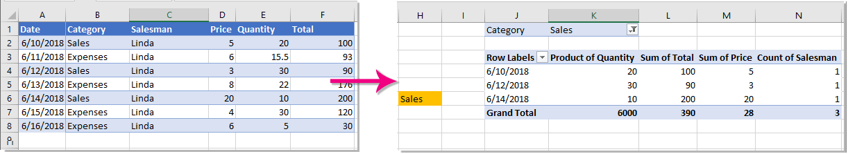
Step 1: Enter the value you want to filter your Pivot Table by into a worksheet cell (for example, type or select the filtering value in cell H6).
Step 2: Open the worksheet that contains your target Pivot Table. Right-click the sheet tab at the bottom of Excel and select View Code from the context menu. This opens the VBA editor window for the worksheet.

Step 3: In the opened Microsoft Visual Basic for Applications (VBA) window, paste the following code into the worksheet’s code module (not a standard module):
VBA code: Filter Pivot Table based on cell value
Private Sub Worksheet_Change(ByVal Target As Range)
'Update by Extendoffice 20180702
    Dim xPTable As PivotTable
    Dim xPFile As PivotField
    Dim xStr As String
    On Error Resume Next
    If Intersect(Target, Range("H6:H7")) Is Nothing Then Exit Sub
    Application.ScreenUpdating = False
    Set xPTable = Worksheets("Sheet1").PivotTables("PivotTable2")
    Set xPFile = xPTable.PivotFields("Category")
    xStr = Target.Text
    xPFile.ClearAllFilters
    xPFile.CurrentPage = xStr
    Application.ScreenUpdating = True
End Sub
📝 Notes:
- "Sheet1" is the worksheet containing the Pivot Table. Adjust as needed.
- "PivotTable2" is the name of your Pivot Table. You can find it in the PivotTable Analyze tab.
- "Category" is the field you want to filter. It must match the field name exactly.
- H6 is the filtering cell. Make sure the value matches an item in the filter list.
- Filter values must match character-by-character. Extra spaces or typos can cause errors or blank results.
Step 4: Press Alt + Q to close the VBA editor and return to Excel.
Now, your Pivot Table should automatically filter to display only the data that matches the value entered in cell H6. This macro runs every time the value in H6 changes, making it easy to adjust your data summary dynamically.
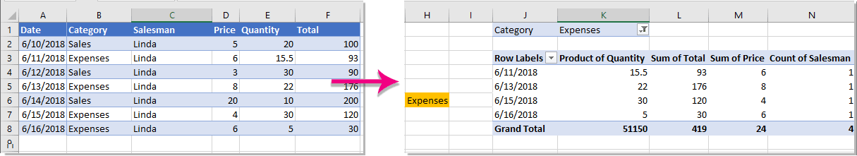
You can modify the value in the filter cell at any time—the Pivot Table will update instantly whenever the cell content is changed or replaced.
Troubleshooting:
- Ensure macros are enabled in your workbook.
- Double-check that the worksheet, Pivot Table, and field names match your actual setup.
- Make sure the filter value in H6 matches the Pivot Table values exactly.
- This VBA approach works for single-field filters. For multiple fields, additional scripting is required.
Excel Formula – Display Filtered Pivot Table Results Based on a Cell Value
For users who prefer not to enable macros, Excel offers formula-based approaches to display Pivot Table results based on a specific cell value. While functions like GETPIVOTDATA and FILTER do not actually change the Pivot Table’s filter settings, they can dynamically reference and present summary results that respond to user input.
This solution is especially useful when building custom summary tables, dashboards, or reports that reflect changing criteria entered by the user—without altering the original Pivot Table view.
Using GETPIVOTDATA:
Suppose your Pivot Table (named "PivotTable2") summarizes sales by category, and the filter value is entered in cell H6. You can use GETPIVOTDATA to display the total sales for the category specified in H6:
1. Select the cell where you want to display the summary result (e.g., I6):
=GETPIVOTDATA("Sum of Sales", $A$4, "Category", $H$6)2. Press Enter. When you change the value in H6, the result in I6 updates automatically to reflect the corresponding summary from the Pivot Table.
If your Pivot Table uses different field names or layout, adjust the formula accordingly. To auto-generate a GETPIVOTDATA formula, type = in a cell, then click on a value cell within your Pivot Table. Excel will insert the appropriate formula, which you can then edit as needed.
Using FILTER with a Helper Table:
If you want to extract detailed records from your original dataset (rather than just Pivot Table summaries), and you are using Excel 365 or Excel 2019, the FILTER function allows dynamic filtering based on a cell value:
Assume your source data is in range A1:C100 and Category is in column A.
1. Select the starting cell where the filtered records should appear (e.g., J6):
=FILTER(A2:C100, A2:A100 = H6, "No data")2. Press Enter. The matching rows will spill into adjacent cells, listing all records where the category matches the value in H6. Updating H6 will instantly refresh the results.
To match Pivot Table groupings or filter on multiple criteria, consider combining GETPIVOTDATA and FILTER, or extend the formula with additional logical conditions.
📝 Tips & Warnings:
- These formulas do not modify the actual Pivot Table filter. They only provide a separate, dynamic view based on cell values.
- To change Pivot Table filters directly, VBA is required.
- Ensure that field names used in
GETPIVOTDATAmatch exactly those in the Pivot Table (case and spacing). - If you see
#REF!errors, verify that your references are valid and the Pivot Table structure hasn't changed.
Other Built-in Excel Methods – Use Slicers as Interactive Pivot Table Filters
If VBA or formula-based solutions don't fully suit your workflow, Excel's Slicers provide another interactive method for filtering Pivot Tables. Slicers are visual filter controls that allow users to filter data with a simple point-and-click interface. While they cannot be linked directly to cell values—meaning you cannot change a cell to control a Slicer—they are intuitive and highly effective for dashboards and reports used by non-technical users.
How to add and use a Slicer:
- Select any cell within your Pivot Table.
- Go to the PivotTable Analyze tab (or Analyze tab in older versions), and click Insert Slicer.
- In the Insert Slicers dialog box, check the field you want to filter by (e.g., Category), then click OK.
- The Slicer will appear on your worksheet. Click a button to filter the Pivot Table by that value. Hold Ctrl to select multiple items.
Slicers can be formatted, resized, and linked to multiple Pivot Tables for synchronized filtering across different reports. They are especially useful in dashboards or shared workbooks where users may not be comfortable with dropdown filters but still need to filter data easily without using VBA or editing formulas.
Limitations: Slicers do not support native linking to cell values. If your workflow requires dynamic filtering controlled by cell input, Slicers should be considered a complementary tool rather than a substitute for VBA or formula-based methods.
Additionally, if your data is stored in an Excel Table (not a Pivot Table), you can still use Slicers by selecting the table and going to the Table Design tab > Insert Slicer.
Troubleshooting: If the Slicer does not appear to filter the Pivot Table, check the Report Connections (under the Slicer or Analyze tab) to ensure it's properly connected to the intended Pivot Table(s).
Each of the methods above serves a different purpose: VBA allows direct cell-linked filtering, formulas provide dynamic display of results, and Slicers offer user-friendly graphical filtering. Choose the approach that best matches your need for automation, flexibility, and ease of use. Traditional Pivot Table dropdown filters remain available as a basic fallback option.
Related articles:
- How to combine multiple sheets into a pivot table in Excel?
- How to create a Pivot Table from Text file in Excel?
- How to link Pivot Table filter to a certain cell in Excel?
Best Office Productivity Tools
Supercharge Your Excel Skills with Kutools for Excel, and Experience Efficiency Like Never Before. Kutools for Excel Offers Over 300 Advanced Features to Boost Productivity and Save Time. Click Here to Get The Feature You Need The Most...
Office Tab Brings Tabbed interface to Office, and Make Your Work Much Easier
- Enable tabbed editing and reading in Word, Excel, PowerPoint, Publisher, Access, Visio and Project.
- Open and create multiple documents in new tabs of the same window, rather than in new windows.
- Increases your productivity by 50%, and reduces hundreds of mouse clicks for you every day!
All Kutools add-ins. One installer
Kutools for Office suite bundles add-ins for Excel, Word, Outlook & PowerPoint plus Office Tab Pro, which is ideal for teams working across Office apps.
- All-in-one suite — Excel, Word, Outlook & PowerPoint add-ins + Office Tab Pro
- One installer, one license — set up in minutes (MSI-ready)
- Works better together — streamlined productivity across Office apps
- 30-day full-featured trial — no registration, no credit card
- Best value — save vs buying individual add-in