Excel INDEX MATCH: Basic and advanced lookups
In Excel, accurately retrieving specific data is often a frequent necessity. While the INDEX and MATCH functions each have their own strengths, combining them unlocks a powerful toolset for data lookup. Together, they facilitate a range of search capabilities, from basic horizontal and vertical lookups to more advanced functionalities like two-way, case-sensitive, and multi-criteria searches. Offering enhanced capabilities compared to VLOOKUP, the pairing of INDEX and MATCH allows for a wider range of data lookup options. In this tutorial, let's delve into the depth of possibilities they can achieve together.
How to use INDEX and MATCH in Excel
Before we use the INDEX and MATCH functions, let’s make sure we know how can INDEX and MATCH help us in looking up values first.
How to use INDEX function in Excel
The INDEX function in Excel returns the value at a given location in a specific range. The syntax of the INDEX function is as follows:
- array (required) refers to the range where you want to return the value from.
- row_num (required, unless column_num is present) refers to the row number of the array.
- column_num (optional, but required if row_num is omitted) refers to the column number of the array.
For example, to know the score of Jeff, the 6th student on the list, you can use the INDEX function like this:
=INDEX(C2:C11,6)
√ Note: The range C2:C11 is where the scores listed, while the number 6 finds the exam score of the 6th student.
Here let’s do a little test. For the formula =INDEX(A1:C1,2), what value will it return? --- Yes, it will return Birth date, the 2nd value in the given row.
Now we should know that the INDEX function can work perfectly with horizontal or vertical ranges. But what if we need it to return a value in a greater range with several rows and columns? Well, in this case, we should apply both a row number and a column number. For example, to find out Jeff's score within the table range instead of a single column, we can locate his score with a row number of 6 and a column number of 3 in the cells through A2 to C11 like this:
=INDEX(A2:C11,6,3)
- The INDEX function can work with vertical and horizontal ranges.
- If both row_num and column_num arguments are used, row_num goes ahead of the column_num, and INDEX retrieves the value at the intersection of the specified row_num and column_num.
However, for a really big database with multiple rows and columns, it’s certainly not convenient for us to apply the formula with an exact row number and column number. And this it when we should combine the use of the MATCH function.

How to use MATCH function in Excel
The MATCH function in Excel returns a numeric value, the location of a specific item in the given range. The syntax of the MATCH function is as follows:
- lookup_value (required) refers to the value to match in the lookup_array.
- lookup_array (required) refers to the range of cells where you want MATCH to search.
- match_type (optional): 1, 0 or -1.
- 1 (default), MATCH will find the largest value that is less than or equal to the lookup_value. The values in the lookup_array must be placed in ascending order.
- 0, MATCH will find the first value that exactly equals the lookup_value. The values in the lookup_array can be in any order. (For the cases that the match type is set to 0, you can use wildcard characters.)
- -1, MATCH will find the smallest value that is greater than or equal to the lookup_value. The values in the lookup_array must be placed in descending order.
For example, to know the position of Vera in the list of names, you can use the MATCH formula like this:
=MATCH("Vera",A2:A11,0)
√ Note: The result “4” indicates that the name “Vera” is in the 4th position of the list.
- The MATCH function returns the position of the lookup value in the lookup array, not the value itself.
- The MATCH function returns the first match in case of duplicates.
- Just like the INDEX function, the MATCH function can work with vertical and horizontal ranges as well.
- MATCH is not case-sensitive.
- If the lookup_value of the MATCH formula is in the form of text, enclose it in quotes.
- If the lookup_value is not found in the lookup_array, the #N/A error is returned.
Now that we know about the basic usages of the INDEX and MATCH functions in Excel, let’s roll up our sleeves and get ready to combine the two functions.
How to combine INDEX and MATCH in Excel
Please see the example below to figure out how can we combine the INDEX and MATCH functions:
To find Evelyn’s score, with the knowledge that the exam scores are in the 3rd column, we can use the MATCH function to automatically determine the row position without the need to manually count it. Subsequently, we can employ the INDEX function to retrieve the value at the intersection of the identified row and the 3rd column:
=INDEX(A2:C11,MATCH("Evelyn",A2:A11,0),3)
Well, since the formula may look a bit complicated, let’s go through each part of it.

The INDEX formula contains three arguments:
- row_num: MATCH("Evelyn",A2:A11,0) provides INDEX with the row position of the value "Evelyn" in the range A2:A11, which is 5.
- column_num: 3 specifies the 3rd column for INDEX to locate the score within the array.
- array: A2:C11 instructs INDEX to return the matching value at the intersection of the specified row and column, within the range spanning from A2 to C11. Finally, we get the result 90.
In the above formula, we employed a hardcoded value, "Evelyn". However, in practice, hardcoded values are impractical, as they would require modification each time we seek to search for different data, such as the score for another student. In such scenarios, we can utilize cell references to create dynamic formulas. For instance, in this case, I will change "Evelyn" to F2:
=INDEX(A2:C11,MATCH(F2,A2:A11,0),3)(AD) Simplify lookups with Kutools: No formula typing required!
Kutools for Excel's Super Lookup provides a variety of lookup tools tailored to meet your every need. Whether you're performing multi-criteria lookups, searching across multiple sheets, or doing one-to-many lookup, Super Lookup simplifies the process with just a few clicks. Explore these features to see how Super Lookup changes the way you interact with Excel data. Say goodbye to the hassle of remembering complex formulas.

Kutools for Excel - Empowering you with over 300 handy functions for effortless productivity. Don't miss your chance to try it out with a 30-day full-featured free trial! Get started now!
INDEX and MATCH formula examples
In this part, we will talk about different circumstances to use the INDEX and MATCH functions to meet different needs.
INDEX and MATCH to apply a two-way lookup
In the previous example, we knew the column number and used a MATCH formula to find the row number. But what if we're unsure about the column number as well?
In such cases, we can perform a two-way lookup, also known as a matrix lookup, by using two MATCH functions: one to find the row number and the other to determine the column number. For example, to know Evelyn’s score, we should use the formula:
=INDEX(A2:C11,MATCH("Evelyn",A2:A11,0),MATCH("Score",A1:C1,0))
- The first MATCH formula finds Evelyn's location in the list A2:A11, providing 5 as the row number to INDEX.
- The second MATCH formula determines the column for the scores and returns 3 as the column number to INDEX.
- The formula simplifies to =INDEX(A2:C11,5,3), and INDEX returns 90.
INDEX and MATCH to apply a left lookup
Now, let's consider a scenario where you need to determine Evelyn's class. You may have noticed that the class column is positioned to the left of the name column, a situation that exceeds the capabilities of another powerful Excel lookup function, VLOOKUP.
In fact, the ability to perform left-side lookups is one of the aspects where the combination of INDEX and MATCH outshines VLOOKUP.
To find Evelyn’s class, employ the following formula to search for Evelyn in B2:B11 and retrieve the corresponding value from A2:A11.
=INDEX(A2:A11,MATCH("Evelyn",B2:B11,0))
Note: You can easily perform a left lookup for specific values using the LOOKUP from Right to Left feature of Kutools for Excel with just a few clicks. To implement the feature, navigate to the Kutools tab in your Excel, and click Super Lookup > LOOKUP from Right to Left in the Formula group.

If you have not installed Kutools, click here to download and get a 30-day full-featured free trial!
INDEX and MATCH to apply a case-sensitive lookup
The MATCH functions is inherently case-insensitive. Yet, when you require your formula to differentiate between upper and lower-case characters, you can enhance it by incorporating the EXACT function. By combining the MATCH function with EXACT in an INDEX formula, you can then effectively perform a case-sensitive lookup, as shown below:
- array refers to the range where you want to return the value from.
- lookup_value refers to the value to match, considering the case of characters, in the lookup_array.
- lookup_array refers to the range of cells where you want MATCH to compare with lookup_value.
For example, to know JIMMY’s exam score, use the following formula:
=INDEX(C2:C11,MATCH(TRUE,EXACT("JIMMY",A2:A11),0))√ Note: This is an array formula that requires you to enter with Ctrl + Shift + Enter, except in Excel 365 and Excel 2021.

- The EXACT function compares "JIMMY" with the values in the list A2:A11, considering the case of characters: If the two strings match precisely, accounting for both upper and lower-case characters, EXACT returns TRUE; otherwise, it returns FALSE. As a result, we obtain an array containing TRUE and FALSE values.
- The MATCH function then retrieves the position of the first TRUE value in the array, which should be 10.
- Finally, INDEX retrieves the value at the 10th position provided by MATCH in the array.
Notes:
- Remember to enter the formula correctly by pressing Ctrl + Shift + Enter, unless you're using Excel 365 or Excel 2021, in which case, simply press Enter.
- The above formula searches within a single list C2:C11. If you want to search within a range with multiple columns and rows, say A2:C11, you should offer both column and row numbers to INDEX:
-
=INDEX(A2:C11,MATCH(TRUE,EXACT("JIMMY",A2:A11),0),3) - In this revised formula, we use the MATCH function to search for "JIMMY", considering the case of characters, in the range A2:A11, and once we find a match, we retrieve the corresponding value from the 3rd column of the range A2:C11.
INDEX and MATCH to find a closest match
In Excel, you might encounter situations where you need to find the nearest or closest match to a specific value within a dataset. In such scenarios, using a combination of INDEX and MATCH functions, along with the ABS and MIN functions, can be incredibly helpful.
- array refers to the range where you want to return the value from.
- lookup_array refers to the the range of values where you want to find the closest match to lookup_value.
- lookup_value refers to the value to find its closest match.
For example, to find out whose score is closest to 85, use the following formula to search for the closest score to 85 in C2:C11 and retrieve the corresponding value from A2:A11.
=INDEX(A2:A11,MATCH(MIN(ABS(C2:C11-85)),ABS(C2:C11-85),0))√ Note: This is an array formula that requires you to enter with Ctrl + Shift + Enter, except in Excel 365 and Excel 2021.

- ABS(C2:C11-85) calculates the absolute difference between each value in the range C2:C11 and 85, resulting in an array of the absolute differences.
- MIN(ABS(C2:C11-85)) finds the minimum value in the array of absolute differences, which represents the closest difference to 85.
- The MATCH function MATCH(MIN(ABS(C2:C11-85)),ABS(C2:C11-85),0) then finds the position of the minimum absolute difference in the array of absolute differences, which should be 10.
- Finally, INDEX retrieves the value at the position in the list A2:A11 that corresponds to the score closest to 85 in the range C2:C11.
Notes:
- Remember to enter the formula correctly by pressing Ctrl + Shift + Enter, unless you're using Excel 365 or Excel 2021, in which case, simply press Enter.
- In case of a tie, this formula will return the first match.
- To find the closest match to the average score, replace 85 in the formula with AVERAGE(C2:C11).
INDEX and MATCH to apply a lookup with multiple criteria
To find a value that meets multiple conditions, requiring you to search across two or more columns, employ the following formula. The formula allows you to perform a multi-criteria lookup by specifying various conditions across different columns, helping you find the desired value that meets all the specified criteria.
√ Note: This is an array formula that requires you to enter with Ctrl + Shift + Enter. A pair of curly brackets will then show up in the formula bar.
- array refers to the range where you want to return the value from.
- (lookup_value=lookup_array) represents a single condition. This condition checks if a particular lookup_value matches the values in the lookup_array.
For example, to find the score of Class A’s Coco, whose birth date is 7/2/2008, you can use the following formula:
=INDEX(D2:D11,MATCH(1,(G2=A2:A11)*(G3=B2:B11)*(G4=C2:C11),0))
Notes:
- In this formula, we avoid hardcoding values, making it simple to obtain a score with different information by modifying the values in cells G2, G3, and G4.
- You should enter the formula by pressing Ctrl + Shift + Enter except in Excel 365 or Excel 2021, where you can simply press Enter.
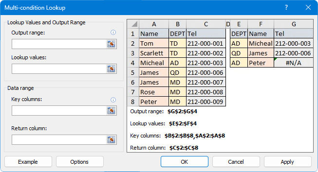
If you constantly forget to use Ctrl + Shift + Enter to complete the formula and get incorrect results, use the following slightly more complex formula, with which you can complete with a simple Enter key:=INDEX(D2:D11,MATCH(1,INDEX((G2=A2:A11)*(G3=B2:B11)*(G4=C2:C11),0,1),0)) - The formulas can be complex and challenging to remember. To simplify multi-criteria lookups without the need for manual formula entry, consider using Kutools for Excel’s Multi-condition Lookup feature. Once you have installed Kutools, navigate to the Kutools tab in your Excel, and click Super Lookup > Multi-condition Lookup in the Formula group.
If you have not installed Kutools, click here to download and get a 30-day full-featured free trial!

INDEX and MATCH to apply a lookup across multiple columns
Imagine a scenario where you're dealing with multiple data columns. The first column acts as a key to classify the data in the other columns. To determine the category or classification for a specific entry, you will have to perform a search across the data columns and associate it with the relevant key in the reference column.
For example, in the table below, how can we match the student Shawn with his corresponding class using INDEX and MATCH? Well, you can achieve it with a formula, but the formula is quite extensive and can be challenging to comprehend, let alone remember and type.
=IFERROR(INDEX($A$2:$A$4,MATCH(IF(SUM(MMULT(--($B$2:$E$4=G2),TRANSPOSE(COLUMN($B$2:$E$4)^0)))>0,1,-1),MMULT(--($B$2:$E$4=G2),TRANSPOSE(COLUMN($B$2:$E$4)^0))^0,0)), "")
That's where Kutools for Excel's Index and Match on Multiple Columns feature comes in handy. It simplifies the process, making it quick and easy to match specific entries with their corresponding categories. To unlock this powerful tool and effortlessly match Shawn with his class, simply download and install the Kutools for Excel add-in, and then do as follows:
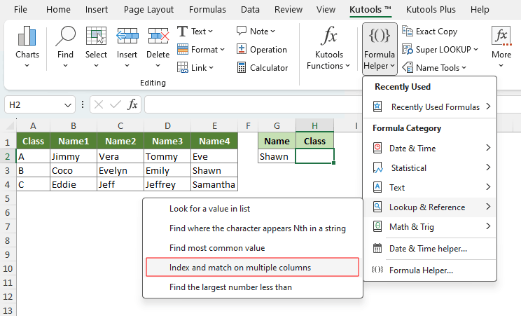
- Select the destination cell where you want to display the matching class.
- On the Kutools tab, click Formula Helper > Lookup & Reference > Index and Match on Multiple Columns.
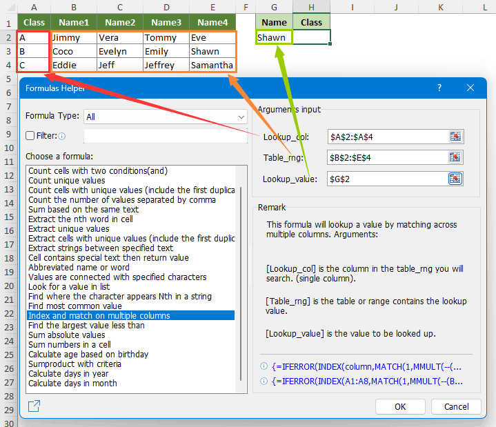
- In the pop-up dialog box, do as follows:
- Click the 1st
 button next to Lookup_col to select the column containing the key information you want to return, i.e., the class names. (You can only select a single column here.)
 - Click the 2nd button next to Table_rng to select the cells to match the values in the selected Lookup_col, i.e., the student names.
- Click the 3rd button next to Lookup_value to select the cell containing the student's name you want to match with their class, in this case, Shawn.
- Click OK.
- Click the 1st


Result
Kutools has automatically generated the formula, and you'll see Shawn's class name displayed in the destination cell immediately.
Note: To try out the Index and Match on Multiple Columns feature, you'll need Kutools for Excel installed on your computer. If you haven't installed it yet, don't wait --- Download and install it now for a 30-day free trial with no limitations. Make Excel work smarter today!
INDEX and MATCH to lookup for first non-blank value
To retrieve the first non-blank value, ignoring errors, from a column or a row, you can use a formula based on INDEX and MATCH functions. However, if you don’t want to ignore the errors from your range, add the ISBLANK function.
- Get first non-blank value in a column or row ignoring errors:
-
=INDEX(B4:B15,MATCH(TRUE,INDEX((B4:B15<>0),0),0)) - Get first non-blank value in a column or row including errors:
-
=INDEX(B4:B15,MATCH(FALSE,ISBLANK(B4:B15),0))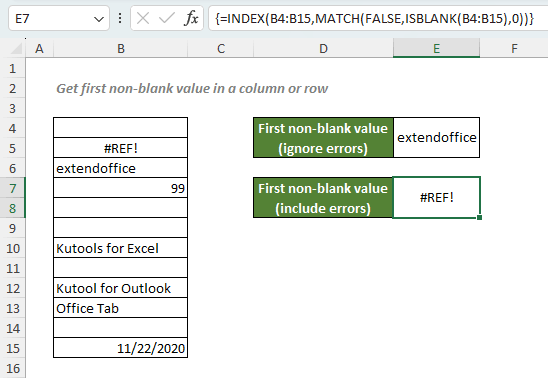

Notes:
- The above are array formulas that require you to enter with Ctrl + Shift + Enter, except in Excel 365 and Excel 2021.
- View this tutorial for a detailed explanation: Get first non-blank value in a column or row.
INDEX and MATCH to lookup for first numeric value
To retrieve the first numeric value from a column or a row, use the formula based on the INDEX, MATCH and ISNUMBER functions.
=INDEX(B4:B15,MATCH(TRUE,ISNUMBER(B4:B15),0))
Notes:
- This is an array formula that requires you to enter with Ctrl + Shift + Enter, except in Excel 365 and Excel 2021.
- View this tutorial for a detailed explanation: Get first numeric value in a column or row.
INDEX and MATCH to lookup for MAX or MIN associations
If you need to retrieve a value associated with the maximum or minimum value within a range, you can use the MAX or MIN function along with the INDEX and MATCH functions.
- INDEX and MATCH to retrieve a value associated with the maximum value:
- =INDEX(array, MATCH(MAX(lookup_array), lookup_array, 0))
- INDEX and MATCH to retrieve a value associated with the minimum value:
- =INDEX(array, MATCH(MIN(lookup_array), lookup_array, 0))
- There are two arguments in the above formulas:
- array refers to the range where you want to return the related information from.
- lookup_array represents the set of values to be examined or searched for specific criteria, i.e., maximum or minimum values.
For instance, if you want to determine who has the highest score, employ the following formula:
=INDEX(A2:A11,MATCH(MAX(C2:C11),C2:C11,0))
- MAX(C2:C11) searches for the highest value in the range C2:C11, which is 96.
- The MATCH function then finds the position of the highest value in the array C2:C11, which should be 1.
- Finally, INDEX retrieves the 1st value in the list A2:A11.
Notes:
- In case of more than one maximum or minimum values, as seen in the example above where two students achieved the same highest score, this formula will return the first match.
- To determine who has the lowest score, use the following formula:
=INDEX(A2:A11,MATCH(MIN(C2:C11),C2:C11,0))
Tip: Tailor your own #N/A error messages
When working with Excel's INDEX and MATCH functions, you may encounter the #N/A error when there's no matching result. For instance, in the table below, when attempting to find the score of a student named Samantha, a #N/A error appears as she is not present in the dataset.

To make your spreadsheets more user-friendly, you can customize this error message by wrapping your INDEX MATCH formula in the IFNA function:
=IFNA(INDEX(C2:C11,MATCH(F2,A2:A11,0)),"Not found")
Notes:
- You can customize your error messages by replacing "Not found" with any text of your choice.
- If you want to handle all errors, not just #N/A, consider using the IFERROR function instead of IFNA:
=IFERROR(INDEX(C2:C11,MATCH(F2,A2:A11,0)),"Not found")Note that it might not be advisable to suppress all errors because they serve as alerts for potential issues in your formulas.
Above is all the relevant content related to the INDEX and MATCH functions in Excel. I hope you find the tutorial helpful. If you're looking to explore more Excel tips and tricks, please click here to access our extensive collection of over thousands of tutorials.
The Best Office Productivity Tools
Kutools for Excel - Helps You To Stand Out From Crowd
Kutools for Excel Boasts Over 300 Features, Ensuring That What You Need is Just A Click Away...
")
Office Tab - Enable Tabbed Reading and Editing in Microsoft Office (include Excel)
- One second to switch between dozens of open documents!
- Reduce hundreds of mouse clicks for you every day, say goodbye to mouse hand.
- Increases your productivity by 50% when viewing and editing multiple documents.
- Brings Efficient Tabs to Office (include Excel), Just Like Chrome, Edge and Firefox.
")
Table of contents
- How to use INDEX and MATCH in Excel
- INDEX function
- MATCH function
- Combine INDEX and MATCH
- INDEX and MATCH examples
- Two-way lookup
- Left lookup
- Case-sensitive lookup
- Closest match
- Lookup with multiple criteria
- Lookup across multiple columns
- Lookup for first non-blank value
- Lookup for first numeric value
- Lookup for MAX or MIN associations
- Tip: Tailor your own #N/A error messages
- The Best Office Productivity Tools
- Comments