Get real-time stock data in Excel: A Rich Data Types guide
In today's digital age, Artificial Intelligence (AI) is revolutionizing the way we handle data. Excel integrates AI into its functionality to help recognize rich data types beyond numbers and text strings, particularly in tracking real-time information such as stock data. Previously, acquiring stock data required manual entry from sources like financial websites or printed materials, which was time-consuming and error prone. Now, real-time stock data can be easily retrieved directly in Excel. This guide will demonstrate how to use the Rich Data Types in Excel to ensure your financial analysis stays up-to-date with the latest market trends.

- Correcting missing data types
- Changing the data types
- Updating the data types
- Discovering more information with cards
Overview of Excel Rich Data Types
With added AI capabilities, rich data types in Excel go beyond the traditional text and numbers. They allow you to bring in a wealth of structured data about various entities. For example, when you enter a company's ticker symbol into a cell and convert it to the Stock data type, Excel fetches a variety of related information, such as stock prices, company names, and more.
What linked data types are available in Excel?
To know what linked data types are available in Excel, go to the "Data" tab in Excel, then you can find the linked data types in the "Data Types" group.

There are 4 data types in the Data Types group, including "Stocks", "Currencies", "Geography" and "Organization". And each one has its associated data types. To know more, visit this page: List of linked data types in Excel.
In this tutorial, I will illustrate how to use the Stocks data type to get real-time stock data.
Accessing Real-Time Stock Data with Rich Data Types
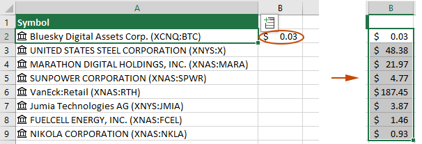
Suppose you have a list of company ticker symbols, as shown in the screenshot below, and want to get the relevant real-time stock information for each of these ticker symbols. This section will demonstrate how to accomplish this task with the Stocks data type in Excel.

Step 1. Convert the original data range to Table
Select the range containing the ticker symbols (in this case, I select the range A1:A9) and press the "Ctrl" + "T" keys. The "Create Table" dialog box will open. You need to check if the cell references are correct and whether your selected range has headers, then click "OK".

Step 2: Convert the ticker symbols to stock data types
Select the original range, go to the "Data" tab, and select "Stocks" in the "Data Types" group.

The selected ticker symbols are converted to stocks data type (a house icon  displays before the texts). See screenshot:

Step 3: Add related information for each ticker symbol
Then you can add real-time information for each ticker symbol. Here I will demonstrate two ways for you.
Method 1: Add fields with the Add Columns button
Click on any cell within the data type, and the "Add Column" button  will appear. And then you need to click this button to show the available fields of data. Click on the field name to extract the information of that field. In this case, I select the "Price" field.

Then the Price field is added to the stock data type. You can repeat this step to add more fields as you need.

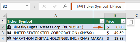
- When you select a cell that contains a field of the rich data type, you can see a formula displayed in the Formula Bar. The data in the selected cell is extracted with this formula.
- If you have not converted the data range to a Table, when adding a field, it will only be applied to the selected data type cell. To populate the field for other data types, you will need to drag the cell’s "Fill Handle" down.


Method 2: Add fields with formulas
If you are familiar with these fields and their corresponding formulas, you can easily add fields using formulas without having to use the Add Column button.
Take the above stocks data type as an example, to add the Price field to this data type, you can do as follows.
- Select a cell to output the field (here I select cell B2), enter the following formula and press the "Enter" key.
=A2.Price
- Select the result cell and double click the Fill Handle (the green square in the lower right corner of the cell) to populate the current column with the same field.


- If the field name to be referenced contains spaces, the field reference needs to be enclosed in square brackets. For example:
=A2.[52 week high] - You can also use the FIELDVALUE function to retrieve field data from linked data types. In this case, the formula should be:
=FIELDVALUE(A2, "Price")
Explore More Options
This section demonstrates additional options that may be used when getting real-time stock data in Excel, including correcting missing data types, changing data types, updating date types, and using Cards to discover more information of the data type.
Correcting Missing Data Types
If Excel does not recognize a ticker, it may fail to convert it into a stock data type. As shown in the screenshot below, Excel does not recognize "Mikecro Soft", so it displays a question mark  before the text. This section will help you correct the missing data type step by step.

- Select the cell containing the missing data type, and the "Data Selector" pane will be displayed automatically.

- In the "Data Selector" pane, you need to do as follow.
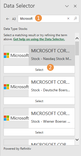
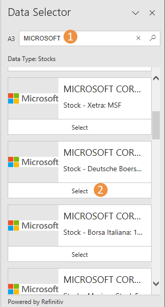
- In such cases, you need to make sure that the ticker symbol is correct. So, try entering the correct ticker symbol in the text box. Here, I changed "Mikecro Soft" to "Microsoft" and then press "Enter" to search for matching results.
- You will then get a list of search results. Select a matching result by clicking on the "Select" button under it.
Tip: You can click on the card above the "Select" button to view the details of this data type.


Result
The missing data type has now been corrected. See screenshot:

Changing the Data Types
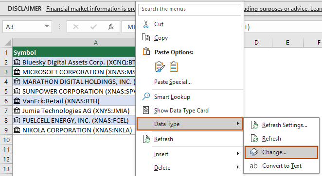
If the data type converted by Excel does not meet your needs, for example, as shown in the screenshot below, the data type in cell A2 is not what you need, you can change it manually as follows.
- Right click on the cell you want to change the data type, select "Data Type" > "Change".
- In the "Data Selector" pane, retype the ticker symbol and press the "Enter" key. Then select the desired data type from the list.


Updating the Data Types
The linked data type connects to an online data source. Once you convert text to a linked data type, an external data connection is established in the workbook. If the online data changes, you will need to manually update the data to get the latest data. This section describes how to update data types in Excel.
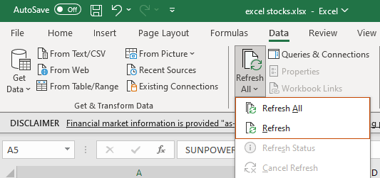
There are three methods you can use to manually update the data types. Click on any cell of the data types, then you need to:
- Right click the selected cell and then select "Refresh" from the context menu.

- Go to the "Data" tab, click "Refresh" > "Refresh All" or "Refresh".
- Use shortcut keys:
- Press "Alt" + "F5" to refresh the cell you selected, as well as other cells with the same data type.
- Press "Ctrl" + "Alt" + "F5" to refresh all sources in the current workbook.


Discovering More Information with Cards
After you convert text into a certain data type, an icon will appear before the text. Clicking the icon will open a card with more detailed information about the data type. Let’s see what we can do with the card.
Click the icon of the data type to open the card. See screenshot:

In the card, you can:
- View all fields and corresponding values of the data type.
- Add desired fields from the card by hovering the cursor over the field and then click the "Extract X to grid" (X here represents the field name).
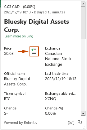
- Know where the fields and values come from by scrolling down inside the card and see the “Powered by” note at the bottom of the card.


Getting Historical Stock Data
The stock data type doesn’t provide historical data. Sometimes, for some purpose, you may need to get historical stock data. This section will briefly describe how to use the STOCKHISTORY function to get historical stock data in Excel for a specific data range.
Syntax of the STOCKHISTORY function
=STOCKHISTORY(stock, start_date, [end_date], [interval], [headers], [property0], [property1], [property2], [property3], [property4], [property5])
Arguments
- Stock (required): A ticker symbol in double quotes, such as "MARA", "JMIA".
- Start_date (required): The start date of the data to be retrieved.
- End_date (optional): The end date of the data to be retrieved. Default is the start_date.
- Interval (optional): The time interval.
- 0 (default) = Daily
- 1 = weekly
- 2 = monthly
- Headers (optional): Specify whether to display headers.
- 0 = No header
- 1 (default) = show header
- 2 = show instrument + header
- Properties (optional): Additional data to retrieve.
- 0 (default) = Date
- 1 (default) = Close
- 2 = Open
- 3 = High
- 4 = Low
- 5 = Volume
Here I will use this function to get the close price of given companies on December 20, 2022.
Select a cell (D2 in this case) next to the original stock list (or select any blank cell you need), enter the following formula and press the "Enter" key.
=STOCKHISTORY(A2,DATE(2022,12,20),,,0)
Select this formula cell and drag its "Fill Handle" down to get the rest of results.

- In this formula, "A2" is the cell with the ticker symbol. "2022,12,20" is the date for retrieving the closing price.
- As I already have headers in my data, I specify the header argument as "0" to avoid displaying extra headers in the results.
- The function returns an array as the result, which includes the specified date for retrieving the closing price, and the closing price for that date.
- To know more about the "STOCKHISTORY function", visit this page on the Microsoft website: STOCKHISTORY function.
FAQs on Utilizing Excel Rich Data Types
Q: How often does Excel update stock data?
A: Excel updates stock data in real-time, though there may be a slight delay for market changes to reflect.
Q: Can I use rich data types for currencies or other financial instruments?
A: Yes, Excel's rich data types also cover currencies and other financial instruments.
Q: Is there a limit to the number of stocks I can track?
A: There's no set limit, but performance might be affected if you're tracking a large number of stocks simultaneously.
Q: Where does the stock financial data come from?
A: To know where the stock financial data comes from, visit this page on the Microsoft website: About the Stocks financial data sources.
Best Office Productivity Tools
Supercharge Your Excel Skills with Kutools for Excel, and Experience Efficiency Like Never Before. Kutools for Excel Offers Over 300 Advanced Features to Boost Productivity and Save Time. Click Here to Get The Feature You Need The Most...
Office Tab Brings Tabbed interface to Office, and Make Your Work Much Easier
- Enable tabbed editing and reading in Word, Excel, PowerPoint, Publisher, Access, Visio and Project.
- Open and create multiple documents in new tabs of the same window, rather than in new windows.
- Increases your productivity by 50%, and reduces hundreds of mouse clicks for you every day!
All Kutools add-ins. One installer
Kutools for Office suite bundles add-ins for Excel, Word, Outlook & PowerPoint plus Office Tab Pro, which is ideal for teams working across Office apps.
- All-in-one suite — Excel, Word, Outlook & PowerPoint add-ins + Office Tab Pro
- One installer, one license — set up in minutes (MSI-ready)
- Works better together — streamlined productivity across Office apps
- 30-day full-featured trial — no registration, no credit card
- Best value — save vs buying individual add-in
Table of contents
- Overview of Excel rich data types
- Accessing real-time stock data
- Explore More Options:
- Correcting missing data types
- Changing the data types
- Updating the data types
- Discovering more with cards
- Getting historical stock data
- FAQs on utilizing Excel Rich Data Types
- Related Articles
- The Best Office Productivity Tools
- Comments