How to vlookup and return the last matching value in Excel?
Excel’s VLOOKUP function is one of the most widely used tools for searching table data based on a specific criterion. By default, however, VLOOKUP can only retrieve the first value that matches your lookup criteria within a dataset. This behavior is often a limitation when your data contains repeated lookup values and you need to extract the last occurrence of a matching entry instead. Such a need frequently arises in scenarios such as tracking the most recent status, finding the latest sales for a customer, or identifying the last recorded entry in chronological lists. To overcome this, Excel offers several alternative approaches utilizing functions like LOOKUP, XLOOKUP, INDEX and MATCH, as well as user-friendly third-party solutions like Kutools for Excel. In this article, we’ll explore how each method works, discuss their practical applications, highlight their strengths and limitations, and provide operation tips to help you vlookup and return the last matching value with ease.
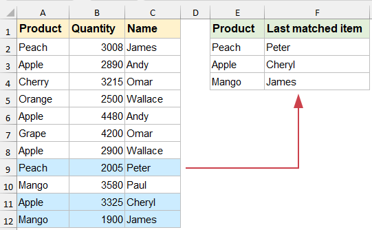
Vlookup and return the last matching value in Excel
Vlookup and return the last matching value with LOOKUP function
Although VLOOKUP cannot directly find the last matching item, the LOOKUP function can offer a clever workaround. The LOOKUP approach is especially handy if your dataset is not sorted and you want a formula-based solution that works in virtually all versions of Excel. This formula leverages the way LOOKUP handles arrays and errors to home in on the last occurrence quickly.
To extract the last matching value using LOOKUP, follow these steps:
1. Select the cell where you want to display the last matching value. Enter the following formula:
=LOOKUP(2,1/($A$2:$A$12=E2),$C$2:$C$12)2. Press Enter. If you need to apply the formula to additional rows, drag the fill handle down to the desired range. This enables you to perform the last-match lookup for multiple search values effortlessly.
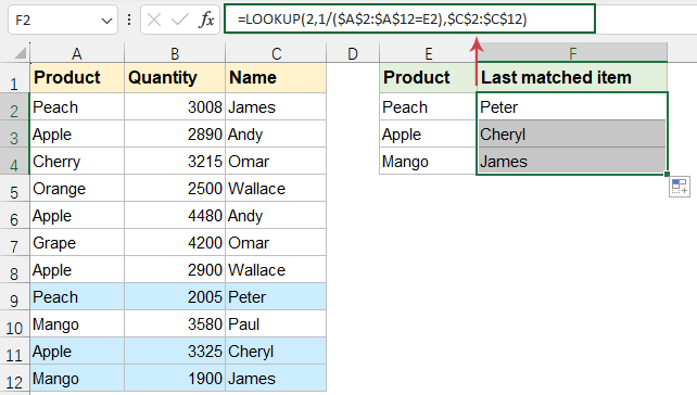
$A$2:$A$12is the lookup column (criteria).E2is the cell containing the value to look up.$C$2:$C$12is the return column (results).
1/($A$2:$A$12=E2)generates an array with a value of 1 where the condition is true, and#DIV/0!errors elsewhere.LOOKUP(2, ...)exploits the fact that LOOKUP ignores errors and searches for the number 2 (which isn’t present). LOOKUP then matches the last 1 in the array and returns the corresponding value from the results array—thus giving the last matching value.
Tips & Notes:
- Ensure the lookup and return ranges have the same size and use absolute references when filling down.
- If the lookup array contains blanks or errors, results may be affected. Clean the data or wrap with
IFERRORas needed. - If you receive
#N/A, confirm the lookup value actually exists in the source range.
Advantages: Works in all Excel versions and avoids special array-entry requirements.
Limitations: Less robust if there are blanks or error values in the lookup array; doesn’t provide custom error outputs without wrapping functions (e.g., IFERROR).
Vlookup and return the last matching value with Kutools for Excel
Kutools for Excel offers an intuitive and efficient way to return the last matching value, ideal for users who prefer a graphical, no-formula approach or need to process large datasets quickly. The built-in LOOKUP from Bottom to Top tool in Kutools' Super LOOKUP suite eliminates formula complexity, auto-handles errors, and can output results to multiple cells simultaneously—saving you time and reducing input mistakes. This method is particularly well suited for users who are not familiar with advanced Excel functions or want to minimize manual formula editing.
After installing Kutools for Excel, follow these steps:
1. Click Kutools > Super LOOKUP > LOOKUP from Bottom to Top. See screenshot:

2. In the LOOKUP from Bottom to Top dialog box:
- Select the lookup value cells and the target output cells in the “Output Range and Lookup values” sections.
- Specify the corresponding data ranges in the “Data range” section. Ensure all ranges match in size and order to avoid misalignment.
- Click OK to apply.


Once executed, Kutools will instantly return the last matching items, as shown below:

Tip: If you want to display a custom message instead of #N/A for unmatched lookups, click Options, check Replace #N/A error value with a specified value, and enter your preferred text.

Pros: No formula editing required. Supports bulk operations and error replacement. Friendly for Excel beginners and suitable for large data tasks.
Cons: Requires the Kutools add-in to be installed; the feature is available only in full or trial versions of Kutools.
Practical Tip: Always review the output and input ranges before confirming to ensure results are accurate, especially if your data changes dynamically.
Vlookup and return the last matching value with INDEX and MATCH functions
The combination of INDEX and MATCH functions provides another flexible and cross-version method to vlookup the last matching value in Excel. This approach is highly adaptable, doesn’t require data sorting, and is compatible with all Excel versions, including legacy editions. However, depending on your Excel version, you may need to use an array formula for correct results.
To use this method, do the following:
1. In your target cell, enter the formula below:
=INDEX($C$2:$C$12,MATCH(2,1/($A$2:$A$12=E2)))2. Confirm the formula:
- In Excel 2019 or earlier, finish with Ctrl + Shift + Enter (Excel will add curly braces {} automatically).
- In Microsoft 365 / Excel 2021 and later, simply press Enter.
3. If you have multiple lookup values, drag the fill handle down to apply the formula to adjacent rows for batch processing.
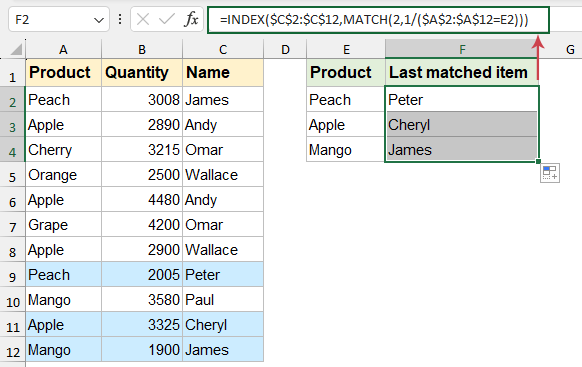
$A$2:$A$12is the lookup column (criteria).E2is the cell containing the value to look up.$C$2:$C$12is the return column (results).
1/($A$2:$A$12=E2)generates an array with a value of 1 where the lookup condition is true, and#DIV/0!errors elsewhere. This converts logical TRUE/FALSE to numeric signals.MATCH(2, 1/($A$2:$A$12=E2))asks Excel to find the number 2 (which isn’t present). MATCH then returns the position of the last 1 in the array—that is, the last true match.INDEX($C$2:$C$12, ...)uses that position to fetch the corresponding value from the return range.
Advice & Tips:
- Ensure the lookup and return ranges have the same number of rows and use absolute references when filling down.
- If you see
#N/Aor#DIV/0!, check for unmatched keys, blanks, or errors in the lookup array. For cleaner output, wrap withIFERROR, e.g.,=IFERROR(your_formula, "").
Advantages: Versatile and backward compatible with all Excel versions.
Drawbacks: Slightly harder to remember; requires array entry in older Excel versions.
Vlookup and return the last matching value with XLOOKUP function
The XLOOKUP function, available in Excel 365, Excel 2021 and later, offers the most straightforward and modern solution for returning the last match. With parameters that control lookup direction and error handling, XLOOKUP can search from the bottom up, retrieving the last matching value without complicated legacy array formulas.
To use XLOOKUP for the last matching value:
1. In your target cell, enter the formula below. Then drag the fill handle if you need it for additional lookup values.
=XLOOKUP(E2, $A$2:$A$12, $C$2:$C$12, , , -1)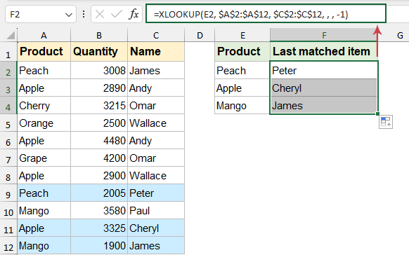
E2: the lookup value.$A$2:$A$12: the lookup array to search.$C$2:$C$12: the return array., ,: two commas indicate the optionalif_not_foundandmatch_modeare omitted (use defaults).-1:search_mode=-1searches from last to first (bottom to top) so you get the last match.
Practical Notes:
- No special array entry is required. You can supply a custom message via
if_not_foundif needed. - XLOOKUP returns the last match based on the order of the provided array (bottom to top with
-1), regardless of filter visibility. - For batch processing, fill down; each row evaluates independently.
Benefits: Simple syntax; built-in last-to-first search; no legacy array formulas.
Limitation: Available only in Excel 365, Excel 2021, and later versions.
Vlookup and return the last matching value with VBA Macro
In some cases, especially if you need to automate the lookup process or work with very large datasets, using a VBA macro can be a practical solution. VBA allows you to custom-script the lookup logic and handle exceptions or special conditions that formulas may not easily address.
Applicable Scenario: Prioritize this solution if you frequently need to run the same lookup operation across different workbooks or want to encapsulate your logic in a reusable script.
1. Click Developer > Visual Basic to open the Microsoft Visual Basic for Applications window. Then click Insert > Module, and paste the following code into the module:
Option Explicit

Sub FindLastMatch()
    Dim searchRange As Range
    Dim returnRange As Range
    Dim searchValue As Variant
    Dim i As Long
    Dim foundValue As Variant
    Dim found As Boolean

    Const xTitleId As String = "KutoolsforExcel"

    ' Get ranges and value from user
    On Error GoTo CleanFail
    Set searchRange = Application.InputBox("Select the lookup column (single column):", xTitleId, Type:=8)
    If TypeName(searchRange) = "Boolean" Then Exit Sub  ' Cancel pressed

    Set returnRange = Application.InputBox("Select the return column (single column):", xTitleId, Type:=8)
    If TypeName(returnRange) = "Boolean" Then Exit Sub  ' Cancel pressed

    searchValue = Application.InputBox("Enter the lookup value:", xTitleId, Type:=2)
    If VarType(searchValue) = vbBoolean And searchValue = False Then Exit Sub  ' Cancel pressed

    ' Basic validations
    If searchRange.Columns.Count <> 1 Or returnRange.Columns.Count <> 1 Then
        MsgBox "Please select a single column for both lookup and return ranges.", vbExclamation
        Exit Sub
    End If

    If searchRange.Rows.Count <> returnRange.Rows.Count Then
        MsgBox "Lookup and return ranges must have the same number of rows.", vbExclamation
        Exit Sub
    End If

    If Not searchRange.Parent Is returnRange.Parent Then
        MsgBox "Lookup and return ranges must be on the same worksheet.", vbExclamation
        Exit Sub
    End If

    ' Scan from bottom to top
    found = False
    For i = searchRange.Rows.Count To 1 Step -1
        If CStr(searchRange.Cells(i, 1).Value) = CStr(searchValue) Then
            foundValue = returnRange.Cells(i, 1).Value
            found = True
            Exit For
        End If
    Next i

    If found Then
        MsgBox "The last matching value is: " & foundValue, vbInformation
    Else
        MsgBox "No match found.", vbInformation
    End If
    Exit Sub

CleanFail:
    MsgBox "Operation cancelled or invalid selection.", vbExclamation
End Sub
2. Click the ![]() button to run the code. In the dialog boxes that appear, select the lookup column, the return column, and enter your lookup value as prompted. The macro scans from the last row upwards and displays the last matching value found.
button to run the code. In the dialog boxes that appear, select the lookup column, the return column, and enter your lookup value as prompted. The macro scans from the last row upwards and displays the last matching value found.
Notes:
- Ensure the lookup and return ranges are single columns, have the same number of rows, and reside on the same worksheet.
- The macro compares values as text for simplicity. If you must distinguish numeric formats (e.g., 00123 vs 123), adjust the comparison logic accordingly.
- If no match is found or the selection is invalid/cancelled, a notification is shown.
Pros: Fully automated, reusable, no need to enter or copy formulas across cells.
Cons: Slightly more complex initial setup; requires a macro-enabled workbook (.xlsm) and trusted macros environment.
Returning the last matching value in Excel is a common requirement—whether you’re monitoring the latest transactions, analyzing updates, or tracking changes over time. With the methods above, you can choose the right approach based on your version of Excel, your workflow preferences, and your familiarity with Excel’s toolset. The LOOKUP, INDEX & MATCH, XLOOKUP, Kutools, and VBA macro approaches each have their own strengths and best-use scenarios.
Troubleshooting: If your formula returns a #N/A or #DIV/0! error, check for incorrect range selection, ensure the lookup value exists, and confirm that your ranges are aligned properly. Avoid empty cells within your lookup column when possible for formula reliability. When in doubt, try out the formula on a small sample of your data to verify your setup—this helps isolate potential mistakes.
For further exploration of lookup techniques—such as retrieving multiple results, concatenating matches, or searching across worksheets—consider visiting specialist resources like our Excel tutorials page for a wide array of related articles and step-by-step guides. Mastering these lookup skills will help you gain confidence in processing, analyzing, and reporting your critical data in Excel more effectively.
More relative articles:
- Vlookup Values Across Multiple Worksheets
- In excel, we can easily apply the vlookup function to return the matching values in a single table of a worksheet. But, have you ever considered that how to vlookup value across multiple worksheet? Supposing I have the following three worksheets with range of data, and now, I want to get part of the corresponding values based on the criteria from these three worksheets.
- Use Vlookup Exact And Approximate Match In Excel
- In Excel, vlookup is one of the most important functions for us to search a value in the left-most column of the table and return the value in the same row of the range. But, do you apply the vlookup function successfully in Excel? This article, I will talk about how to use the vlookup function in Excel.
- Vlookup To Return Blank Or Specific Value Instead Of0 Or N/A
- Normally, when you apply the vlookup function to return the corresponding value, if your matching cell is blank, it will return0, and if your matching value is not found, you will get an error #N/A value as below screenshot shown. Instead of displaying the0 or #N/A value, how can you make it show blank cell or other specific text value?
- Vlookup And Return Whole / Entire Row Of A Matched Value In Excel
- Normally, you can vlookup and return a matching value from a range of data by using the Vlookup function, but, have you ever tried to find and return the whole row of data based on specific criteria as following screenshot shown.
- Vlookup And Concatenate Multiple Corresponding Values In Excel
- As we all known, the Vlookup function in Excel can help us to lookup a value and return the corresponding data in another column, but in general, it can only get the first relative value if there are multiple matching data. In this article, I will talk about how to vlookup and concatenate multiple corresponding values in only one cell or a vertical list.
Best Office Productivity Tools
Supercharge Your Excel Skills with Kutools for Excel, and Experience Efficiency Like Never Before. Kutools for Excel Offers Over 300 Advanced Features to Boost Productivity and Save Time. Click Here to Get The Feature You Need The Most...
Office Tab Brings Tabbed interface to Office, and Make Your Work Much Easier
- Enable tabbed editing and reading in Word, Excel, PowerPoint, Publisher, Access, Visio and Project.
- Open and create multiple documents in new tabs of the same window, rather than in new windows.
- Increases your productivity by 50%, and reduces hundreds of mouse clicks for you every day!
All Kutools add-ins. One installer
Kutools for Office suite bundles add-ins for Excel, Word, Outlook & PowerPoint plus Office Tab Pro, which is ideal for teams working across Office apps.
- All-in-one suite — Excel, Word, Outlook & PowerPoint add-ins + Office Tab Pro
- One installer, one license — set up in minutes (MSI-ready)
- Works better together — streamlined productivity across Office apps
- 30-day full-featured trial — no registration, no credit card
- Best value — save vs buying individual add-in