How to select the highest or lowest value in Excel?

Sometime you may need to find out and select the highest or lowest values in a spreadsheet or a selection, such as the highest sales amount, lowest price, etc. how do you deal with it? This article brings you some tricky tips to find out and select the highest values and lowest values in selections.


Find out the highest or lowest value in a selection with formulas


To get the largest or smallest number in a range:

Just enter the below formula into a blank cell you want to get the result:

Get the largest value: =Max (B2:F10)
Get the smallest value: =Min (B2:F10)

And then press Enter key to get the largest or smallest number in the range, see screenshot:


To get the largest 3 or smallest 3 numbers in a range:

Sometimes, you may want to find the largest or smallest 3 numbers from a worksheet, this section, I will introduce formulas for you to solve this problem, please do as follows:

Please enter below formula into a cell:

Get the largest 3 values: =LARGE(B2:F10,1)&", "&LARGE(B2:F10,2)&", "&LARGE(B2:F10,3)
Get the smallest 3 values: =SMALL(B2:F10,1)&", "&SMALL(B2:F10,2)&", "&SMALL(B2:F10,3)

  • Tips: If you want to find the largest or smallest 5 numbers, you just need to use the & to join the LARGE or SMALL function like this:
  • =LARGE(B2:F10,1)&", "&LARGE(B2:F10,2)&", "&LARGE(B2:F10,3)&","&LARGE(B2:F10,4) &","&LARGE(B2:F10,5)

Tips: Too difficult to remember these formulas, but if you have the Auto Text feature of Kutools for Excel, it helps you to save all formulas you need, and reuse them at anywhere anytime as you like.     Click to download Kutools for Excel!


Find and highlight the highest or lowest value in a selection with Conditional Formatting

Normally, the Conditional Formatting feature also can help to find and select the largest or smallest n values from a range of cells, please do as this:

1. Click Home > Conditional Formatting > Top/Bottom Rules > Top 10 Items, see screenshot:

2. In the Top 10 Items dialog box, enter the number of largest values that you want to find, and then choose one format for them, and the largest n values have been highlighted, see screenshot:

  • Tips: To find and highlight the lowest n values, you just need to Click Home > Conditional Formatting > Top/Bottom Rules > Bottom 10 Items.

Select all of the highest or lowest value in a selection with a powerful feature

The Kutools for Excel's Select Cells with Max & Min Value will help you not only find out the highest or lowest values, but also select all of them together in selections.

Tips:To apply this Select Cells with Max & Min Value feature, firstly, you should download the Kutools for Excel, and then apply the feature quickly and easily.

After installing Kutools for Excel, please do as this:

1. Select the range that you will work with, then click Kutools > Select > Select Cells with Max & Min Value…, see screenshot:

3. In the Select Cells with Max & Min Value dialog box:

  • (1.) Specify the type of cells to search (formulas, values, or both) in the Look in box;
  • (2.) Then check the Maximum value or Minimum value as you need;
  • (3.) And specify the scope that the largest or smallest based on, here, please choose Cell.
  • (4.) And then if you want to select the first matching cell, just choose the First cell only option, to select all the matching cells, please choose All cells option.

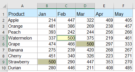
4. And then click OK, it will select all highest values or lowest values in the selection, see the following screenshots:

Select all the smallest values

Select all the largest values
Download and free trial Kutools for Excel Now!


Select the highest or lowest value in each row or column with a powerful feature

If you want to find and select the highest or lowest value in each row or column, the Kutools for Excel also can do you a favor, please do as follows:

1. Select the data range that you want to select the largest or smallest value. Then click Kutools > Select > Select Cells with Max & Min Value to enable this feature.

2. In the Select Cells with Max & Min Value dialog box, set the following operations as you need:

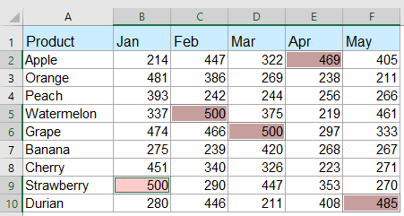
4. Then click Ok button, all the largest or smallest value in each row or column are selected at once, see screenshots:

The largest value in each row

The largest value in each column
Download and free trial Kutools for Excel Now!


Select or highlight all cells with the largest or smallest values in a range of cells or each column and row

With Kutools for Excel's Select Cells with Max & Min Values feature, you can quickly select or highlight all of the largest or smallest values from a range of cells, each row or each column as you need. Please see the below demo.    Click to download Kutools for Excel!


More relative largest or smallest value articles:

  • Find And Get The Nth Largest Value Without Duplicates In Excel
  • In Excel worksheet, we can get the largest, the second largest or nth largest value by applying the Large function. But, if there are duplicate values in the list, this function will not skip the duplicates when extracting the nth largest value. In this case, how could you get the nth largest value without duplicates in Excel?
  • Find The Nth Largest / Smallest Unique Value In Excel
  • If you have a list of numbers which contains some duplicates, to get the nth largest or smallest value among these numbers, the normal Large and Small function will return the result including the duplicates. How could you return the nth largest or smallest value ignoring the duplicates in Excel?
  • Highlight Largest / Lowest Value In Each Row Or Column
  • If you have multiple columns and rows data, how could you highlight the largest or lowest value in each row or column? It will be tedious if you identify the values one by one in each row or column. In this case, the Conditional Formatting feature in Excel can do you a favor. Please read more to know the details.
  • Sum Largest Or Smallest 3 Values In A List Of Excel
  • It is common for us to add up a range of numbers by using the SUM function, but sometimes, we need to sum the largest or smallest 3, 10 or n numbers in a range, this may be a complicated task. Today I introduce you some formulas to solve this problem.

Best Office Productivity Tools

Supercharge Your Spreadsheets: Experience Efficiency Like Never Before with Kutools for Excel

Popular Features: Find/Highlight/Identify Duplicates   |  Delete Blank Rows   |  Combine Columns or Cells without Losing Data   |   Round without Formula ...
Super Lookup: Multiple Criteria VLookup    Multiple Value VLookup  |   VLookup Across Multiple Sheets   |   Fuzzy Lookup ....
Advanced Drop-down List: Quickly Create Drop Down List   |  Dependent Drop Down List   |  Multi-select Drop Down List ....
Column Manager: Add a Specific Number of Columns     Move Columns   |   Unhide Columns   |   Compare Columns to Select Same & Different Cells ...
Featured Features: Grid Focus   |  Design View   |   Big Formula Bar    Workbook & Sheet Manager   |  Resource Library (Auto Text)   |  Date Picker   |  Combine Worksheets   |  Encrypt/Decrypt Cells    Send Emails by List   |  Super Filter   |   Special Filter (filter bold/italic/strikethrough...) ...
Top 15 Toolset12 Text Tools (Add Text, Remove Characters, ...)   |   50+ Chart Types (Gantt Chart, ...)   |   40+ Practical Formulas (Calculate age based on birthday, ...)   |   19 Insertion Tools (Insert QR Code, Insert Picture from Path, ...)   |   12 Conversion Tools (Numbers to Words, Currency Conversion, ...)   |   7 Merge & Split Tools (Advanced Combine Rows, Split Cells, ...)   |   Many More...

Kutools for Excel boasts over 300 features, ensuring that what you need is just a click away...

Supports Office/Excel 2007-2021 & newer, including 365   |   Available in 44 languages   |   Enjoy a full-featured 30-day free trial.

kte tab 201905


Office Tab Brings Tabbed interface to Office, and Make Your Work Much Easier

  • Enable tabbed editing and reading in Word, Excel, PowerPoint, Publisher, Access, Visio and Project.
  • Open and create multiple documents in new tabs of the same window, rather than in new windows.
  • Increases your productivity by 50%, and reduces hundreds of mouse clicks for you every day!
Comments (39)
Rated 5 out of 5 · 1 ratings
This comment was minimized by the moderator on the site
Hi, any idea why this formula does not work: =MAX(B5,B8,B11,B14)-MIN(B5,B8,B11,B14)

=MAX(B5:B14)-MIN(B5:B14) works but I want just the four cells, not the whole range...
This comment was minimized by the moderator on the site
Hi there,

The formula should work. Is there anything wrong with the data type?

Amanda
This comment was minimized by the moderator on the site
Hi, can u help me. i got some problem on how to retrieve which outlet got lowest growth percentage since the percentage got duplicate value

for example

PEN001 -83.33%
PEN002 -83.33%
PEN003 -92.31%
PEN004 -100.00%
PEN005 -100.00%

I'm using index match min (lowest) & small (for 2nd lowest), but the result will return PEN004 for both condition which is the lowest and 2nd lowest
This comment was minimized by the moderator on the site
Hi,

To ignore the duplicate values and only count unique values, you can use the formula below:
=INDEX(A1:A6,MATCH(SMALL(IF(ISNUMBER(B1:B6),IF(ROW(B1:B6)=MATCH(B1:B6,B1:B6,0),B1:B6)),2),B1:B6,0))

In the above formula, A1:A6 is the list of PEN00N, B1:B6 is the list of percentages, 2 means to get the 2nd lowest value.
https://www.extendoffice.com/images/stories/comments/ljy-picture/2nd_unique_lowest_value.png

Note that this formula works for unique values only, which means it will only return the first value if there are duplicates.

Amanda
This comment was minimized by the moderator on the site
Cześć,

Potrzebuje poznać sposób na rozbudowanie komendy max/min by w docelowej komórce pokazywała wartość wraz z kolorem komórki.

Przykład
mam 3 dostawców z różnymi cenami tych samych produktów (produkty pionowo, dostawcy poziomo)
Dostawcy są przykładowo w kolumnach E,F,G i każdemu przydzieliłem inny kolor, który obowiązuje również ceny danego dostawcy.
W komórkach H chciałbym by pokazała się najniższa cena wraz z kolorem danego dostawcy.

dzięki!
This comment was minimized by the moderator on the site
Hi there,

Let's say the table is as shown below, you could use Excel's Conditional formatting to get the result you want:
https://www.extendoffice.com/images/stories/comments/ljy-picture/example.png

1. Enter =MIN(E1:G1,I1) in cell H1, and then copy the formula to below cells.
https://www.extendoffice.com/images/stories/comments/ljy-picture/get-min.png
2. Selet the list H1: H5, and then on the Home tab, click Conditional Formatting > New rule.
3. In the dialog box, selet Use a formula to determine which cells to format; Enter =$H1=$E1; And then click on Format to choose the background color of cell E1.
https://www.extendoffice.com/images/stories/comments/ljy-picture/create-rule.png
4. Repeat the step 3 to create rules for other background colors: =$H1=$F1 > light blue; =$H1=$G1 > light green; ...

Now, your table should look like this:
https://www.extendoffice.com/images/stories/comments/ljy-picture/result.png

Amanda
This comment was minimized by the moderator on the site
I have a table and I need to sum the columns(which I have done) then I need to find the lowest value (which I have done) how do I display the column title of the lowest value?

Thanks
This comment was minimized by the moderator on the site
Hi, could you please show me a screenshot of your data?

Amanda
This comment was minimized by the moderator on the site
Bonjour Amanda

Ca marche !!!! 😀 🤩 👌
Merci vraiment

Puis-je vous demander de nouveau votre aide ?
Voici la formule que je recherche

A1 A2 A3 A4
Chien Colibri Renard OK
Chat Renard Chien OK
Souris Chien Lion Non
Colibri Ecureuil Marmotte Non
Eléphant Colibri Chat OK

Si en A3 on retrouve les mots des colonnes A1 et A2 alors la colonne A4 indique OK
Si en A3 on ne retrouve pas les mots des colonnes A1 et A2 alors la colonne A4 indique Non

Merci encore pour votre aide très précieuse pour une débutante en excel

Bonne journée
Rated 5 out of 5
This comment was minimized by the moderator on the site
Hi, I don't quite understand why did you asign OK to the first and second rows, since I don't see that the third value is the same as the first or second one.

Amanda
This comment was minimized by the moderator on the site
Bonjour Amanda,

Je vous ai renvoyé le fichier à l'adresse mail indiquée : à l'instant

Merci encore une fois de votre aide.

Bien cordialement
This comment was minimized by the moderator on the site
Hi there,

I tried your excel file in the French enviorment, please use =IF(A1=MAX($A$1:$A$4);1;0).
The seperator should be ";" instead of "," 😅
(If the formula does not work, use SI instead of IF)

Amanda
This comment was minimized by the moderator on the site
Bonjour Amanda

Ne pouvons joindre de fichier sur le site, j'ai répondu au mail que vous m'avez envoyé et j'y ai joins le fichier excel
Vous pourrez voir ainsi que cela me mets en erreur.

Merci encore de votre aide

Bien cordialement
This comment was minimized by the moderator on the site
Hi there,

Did you send the excel file to ?
I did not receive any messages about the issue. Could you please send that again?
Also, I think the .xlsx file is supported to upload here. If you want, you can just upload it here in a comment.

Amanda
This comment was minimized by the moderator on the site
Bonjour,
En premier lieu merci pour tout ça j'y ai trouvé plein plein de soluces.
Ma question est la suivante
J'ai une colonne avec des chiffres

26.56250
25.10400
26.29101
27.66667

Et je voudrais en parallèle une formule qui va me dire non seulement le nombre le plus élevé (ça j'ai trouvé dans vos explications) mais que cette colonne indique 1 pour le chiffre le plus élevé.
Voici un exemple

26.56250 = 0
25.10400 = 0
26.29101 = 0
27.66667 = 1

Pensez-vous que cela soit possible et si oui via quelle formule ?

Je vous remercie encore et par avance en + 😄

Bien cordialement
This comment was minimized by the moderator on the site
Hi there,

Let's say the four values are in range A1:A4, you can enter the below formula in B1:
=IF(A1=MAX($A$1:$A$4),1,0)
And then drag the fill handle down to apply the formula to below cells.
https://www.extendoffice.com/images/stories/comments/ljy-picture/return-1-if-max.png

Amanda
This comment was minimized by the moderator on the site
Bonjour Amandine
Tout d'abord merci pour cette réponse.
Malheureusement cela ne fonctionne pas <font style="vertical-align: inherit;"><font style="vertical-align: inherit;">😞</font></font>

J'ai le message d'erreur habituel
Pouvez-vous m'aider encore une fois ?

Merci
This comment was minimized by the moderator on the site
Hi there,

Can tell me what error it is? I noticed that you are using French, so please try SI instead of IF: =SI(A1=MAX($A$1:$A$4),1,0)

Amanda
This comment was minimized by the moderator on the site
Good day
I have difficulty with excel and don't know the exact names of what I want but will give it a try ?

1. I have 4 Colom's A, B, C, D, =MAX()
9, 2, 4, 1,
I want a formula that include the A,B,C,D, for instance, want the formula to include the "A" and "9" as well like A9?


2 A, B, C, D,
9, 8, 9, 2,
I also need a formula for if there is 2 (or 3 or even 4) equals highs, where I can "A9" and "C9" selected as highest ?

3 base on this information how can I create an automated report for the login user once they have selected the highest value ?

4. Maybe this is not the place to ask, but how can I create a time limit for the usage of the excel workbook that expires after 30 minutes and automatically email the report
to the login user?

5. lastly the report that the user will receive is in word format

Thank you so much
Have a wonderful day
This comment was minimized by the moderator on the site
How do I write a formula to find the smallest percentage in these 3 columns and return the value as LAG Alt or GDF or DEL?
LAG ALT -5% GDF -32% DEL 28%

In example above LAG ALT is the smallest percent/Choice I would want
This comment was minimized by the moderator on the site
Hi, the value to be compared and text string have to be in two cells for excel to compre. I have wrote a formula to get the result you want: =INDEX(A2:C2,MATCH(MIN(ABS(A3:C3)),ABS(A3:C3),0)) Please refer to the screenshot to see how it works. For more details about the formula, please click the link below. I only added ABS function (to get the absolute value) to the formula listed in the article: https://www.extendoffice.com/excel/formulas/excel-get-information-corresponding-to-minimum-value.html
This comment was minimized by the moderator on the site
Im trying to create a price benchmarking tool on a separate sheet from my data table.  Data table has customers across the top, skus down the side, and their prices at the intersections (way too many SKUs to put those across the top and I have too many other functions running off of this table to change course).  I'm using large and small functions to get the highest and lowest 3 values, and have those values being calculated directly into my data table.  I'm pulling them into the other sheet using a vlookup on that table referencing the sku number and those specific columns.  I can return the row number where those values are found using a Match function that references the SKU, but cant figure out how to return the column where the actual price is specific to that returned value for the row.  Thinking that there's a simpler way to do this that I'm just not aware of or am missing.
This comment was minimized by the moderator on the site
Ik heb cellen waarin een aantal waarden opgeteld worden, dus =4,25+1,5+,25.Ik zoek een formule die het maximum/minimum uit die cel haalt. Is dat mogelijk? Ik gebruik Excel 2010.
This comment was minimized by the moderator on the site
need to extract smaller amount from two rows for example
51000
5000
smaller amount should cut and paste to next line.
it should continue the whole sheet.. the common thing is 0 after each two amounts and it should skip if there is only one number ( 0, 250, 0) like below blow example
51000
5000
0
10000
1000
0250031003000300000
This comment was minimized by the moderator on the site
This might be very specific, but is there a way to show the title thats all the way to the left of the highest value?
So like this:

Example1: 3 | Example3 has the highest value.
Example2: 2 | -
Example3: 4 | -
Example4: 1 | -
This comment was minimized by the moderator on the site
Hi, Dirk,
To solve your problem, please apply the following formula:
=INDEX(A1:A7,MATCH(MAX(B1:B7),B1:B7,FALSE),)&" has the highest value: "&MAX(B1:B7)
see the below screenshot.

Please try, hope it can help you!
This comment was minimized by the moderator on the site
Hi all

i need to extract data in a range, this formula is working fine but its not showing duplicate values. is there any chance that i get duplicate value too?

=INDEX($B$36:$V$36,MATCH(1,INDEX(($B$36:$V$36=LARGE($B$36:$V$36,ROWS(AB$7:AB13)))*(COUNTIF(AB$7:AB13,$B$36:$V$36)=0),),0))
This comment was minimized by the moderator on the site
Hi, Arslan,
Can you give the more detialed information of your problem, or you can insert a screenshot here. Thank you!
This comment was minimized by the moderator on the site
I have an excel sheet with various columns - Date - Item Names - Qty - Price - Total Price. This item was purchased on many dates with different price. How to find out maximum price for each item ?
This comment was minimized by the moderator on the site
Hi, R NAGARAJAN,
To find the largest value based on criteria, may be the below formula can help you: (please change the cell references to your need)

=MAX(($A$2:$A$10=E2)*$C$2:$C$10) (press Ctrl + Shift + Enter keys together to get the correct results. )
This comment was minimized by the moderator on the site
hi, skyyang
thanks for your formula, it works. finally can you help me to get Minimum value with criteria?
i used this {=MIN(($F$3:$F$1240=I3)*($H$3:$H$1240))} with ctrl+shift+enter and provides wrong calculation, it shows all 0 value.
This comment was minimized by the moderator on the site
Hi, Azad,
To get the smallest value based on the criteria, please apply the below formula:
=MIN(IF(A2:A11=D2,B2:B11))
Please remember to press ctrl+shift+enter keys together. And change the cell references to your need.

Please try, hope it can help you!
This comment was minimized by the moderator on the site
Hello dear thank you very much it works.
This comment was minimized by the moderator on the site
How would I format the numbers that are returned?
This comment was minimized by the moderator on the site
How would I format the numbers that are returned?
This comment was minimized by the moderator on the site
dear sir,
how to find MAX and MIN in this images (in place of 1,2,3,4,5,6,7,8,9,10)


Max Range
1 =7.00Hrs.
2 =132.88Kv
3= -222.40Amp
4= -43MW
5=-27.07Mvar

Min range


6= 14.00Hrs
7= 136.32Kv
8= -119.20Hrs
9= -2MW
10= -27.84Mvar
This comment was minimized by the moderator on the site
Hi, what if I want to select the lowest 3 values or maximum 3 values, or lowest 1/3 values or max 2/3 values, etc. Is there a way to do this? Thanks!
This comment was minimized by the moderator on the site
First use =counta to count number of cells tha is not empty (x) Then =x/3*2 (y) Then =small(range,y) =small(range,y-1) and so on until u get y-1 =1
This comment was minimized by the moderator on the site
Dear Sir, I am looking for a formulea which can search product-wise. Suppose in in column A, you have 10 of Product A and in column B you have several prices for the same product A. See example below: PRODUCT PRICE Prooduct A 12 Prooduct A 19 Prooduct A 11 Prooduct A 21 Prooduct A 10 Prooduct B 16 Prooduct B 21 Prooduct B 13 Prooduct B 12 Prooduct C 21 Prooduct C 14 Prooduct C 10 Looking for a formulea which can search by product (product-wise). Thanks and best regards,
There are no comments posted here yet
Please leave your comments in English
Posting as Guest
×
Rate this post:
0   Characters
Suggested Locations