Excel SUMIF function
In Excel, the SUMIF function can help to sum cells based on one criterion, this article will explain this function's syntax and introduce some examples for using the SUMIF function.
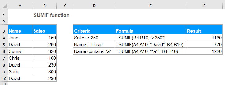
- Example 1: Sum if values are greater than, less than, equal to or other comparison operators
- Example 2: SUMIF formulas with text criteria
- Example 3: SUMIF formulas with wildcard characters
- Example 4: Sum cell values that corresponding to blank or non-blank cells
- Example 5: SUMIF with dates in Excel
- Example 6: Sum values in multiple columns in Excel
Syntax:
The syntax for the SUMIF function in Excel is:
Arguments:
- range: Required. The range of cells that you want to apply the criteria.
- criteria: Required. The criteria used to determine which cells need to add. The criteria can be text, number, date, logical expression, cell reference or another function.
- Note: Any text criteria or criteria containing mathematical symbols must be enclosed in double quotations marks. If the criteria is numeric, double quotation marks are not required.
- sum_range:Optional. It is the range of cells to sum together. If this parameter is omitted, it uses range as the sum_range.
Return:
Return the summation for a list of numbers based on the specific criteria.
Examples:
Example 1: Sum if values are greater than, less than, equal to or other comparison operators
In Excel, you can use the SUMIF function to add up values greater than, less than, equal to or not equal to a given criteria.
Supposing, you have a table which contains Name, Qty and Price columns as below screenshot shown, how could you get the total price that the Qty is greater than 250?
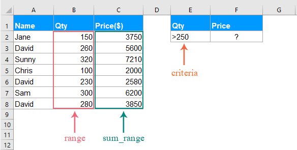
Please apply the below formula into a blank cell:
- Tips: In the above formula:
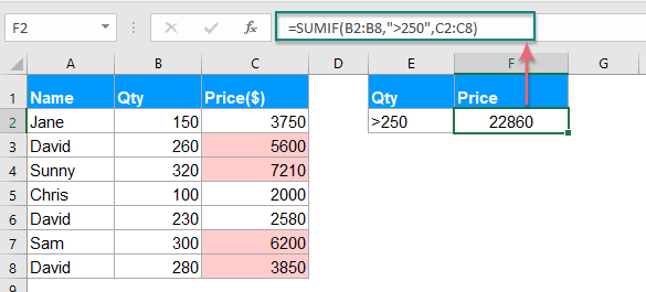
- B2:B8: is the range of cells where the criteria will be looking for.
- ">250": is the condition you want to sum the cell values based on.
- C2:C8: refers to the range to be summed.
Then press Enter key to get the total price that the Qty is greater than 250 as following screenshot shown:
Note: You can use other comparison operators, such as greater than or equal to (>=), less than (<), less than or equal to (<=), equal to (=), not equal to (<>) to your need.
Example 2: SUMIF formulas with text criteria
If you want to sum cell values based on whether a specific text value exists in another column, the SUMIF function also can do you a favor.
Case 1: Sum cell values if contains specific text in another column
Take the below data as example, to get all the total Qty if the name is David in column A.
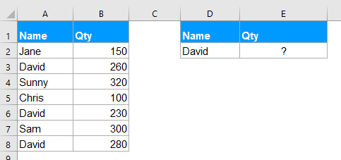
Please enter or copy the below formula into a blank cell:
- Tips: In the above formula:
- A2:A8: is the range of cells where the criteria will be looking for.
- "David": is the condition you want to sum the cell values based on.
- B2:B8: is the range of cells to be summed.
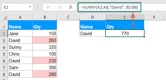
Note: You can also use the cell reference to replace the condition in the above formula as this: =SUMIF(A2:A8, D2, B2:B8).
Case 2: Sum cell values not equal to a specific value
If you want to sum cells when the cells are not equal to a specific value, for example, to sum all Qty of the people except David, how could you do?
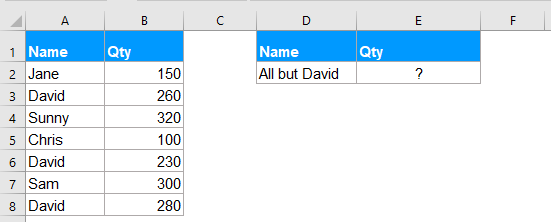
Please apply the below formula into a blank cell:
- Tips: In the above formula:
- A2:A8: is the range of cells where the criteria will be looking for.
- "<>David": is the condition you want to sum the cell values based on.
- B2:B8: is the range of cells to be summed.
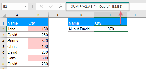
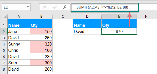
Note: You can also use the cell reference to replace the condition in the above formula as this: =SUMIF(A2:A8,"<>"&D2, B2:B8), you must use the double quotes ("") to enclose the comparison operators and use ampersand (&) to concatenate the cell reference. See screenshot:
Example 3: SUMIF formulas with wildcard characters
Sometimes, you may need to sum the cell values based on partial text match instead of the exact match. In this case, you can combine the wildcard characters asterisk (*) or question mark (?) with the SUMIF function.
Asterisk (*): Represents any number of characters
Question mark (?): Represents anyone single character in a specific position
Case 1: Sum values based on partial match with asterisk (*) character
For instance, I have a table as following screenshot shown, now, I want to sum the total orders of the product which text contains Kutools.
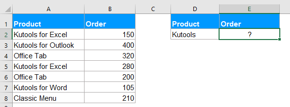
Here, please apply the following formula into a blank cell:
Then, press Enter key to get the below result:
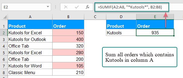
Notes:
1. If you want to sum cell values that the start with Kutools, please use this formula: =SUMIF(A2:A8, "Kutools*", B2:B8).
2. To sum cell values if the corresponding cell in Column A ends with the text Kutools, please use this formula: =SUMIF(A2:A8, "*Kutools", B2:B8).
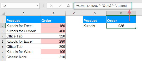
3. You can also use the cell reference to replace the condition in the above formula as this: =SUMIF(A2:A8, "*"&D2&"*", B2:B8). You should use the double quotes ("") to enclose the asterisk and use ampersand (&) to concatenate the cell reference. See screenshot:
Case 2: Sum values with specific number of characters with question mark (?)
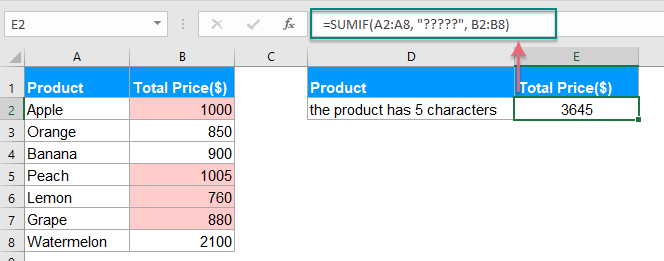
If you want to sum the cell values in a list which corresponding cell has exactly 5 characters long as following screenshot shown. How could you solve this task in Excel?
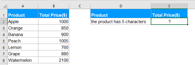
To deal with this job, you should apply the below formula:
Tip: In this formula: one question mark represents one single character, five-question marks indicate 5 characters long.
And then, press Enter key, you will get the result you need:
Example 4: Sum cell values that corresponding to blank or non-blank cells
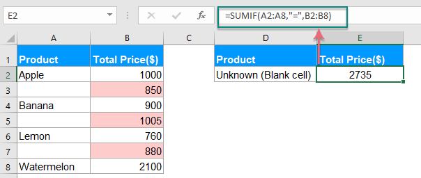
In Excel, the SUMIF function also can help to sum values in a list that the adjacent cell is blank cell or non-blank cells.
Case 1: Sum cell values if adjacent cell is blank
Please enter or copy any one of the below formulas into a cell where you want to get the result:
Then, press Enter key to get the result of the total price if there are blank cells in Column A, see screenshot:
Case 2: Sum cell values if adjacent cell is non-blank cell
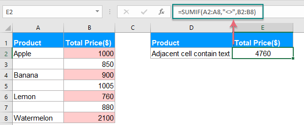
If you need to sum values where the adjacent cells contain texts excluding blank cells, please apply the below formula:
And then, press Enter key, all values where the adjacent cells contain values have been summed together, see screenshot:
Example 5: SUMIF with dates in Excel
Normally, you can also use the SUMIF function to sum values based on specific date in Excel.
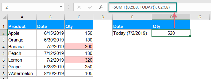
Case 1: Sum values if date is current date or less than, greater than today
To sum the cell values which date is current date, you can use the below formula:
Then, press Enter key, all the cells that the corresponding date is today are summed. See screenshot:
Notes:
1. To sum the values if the corresponding date is less than or before today, please use this formula: =SUMIF(B2:B8, "<"&TODAY(), C2:C8).
2. To sum the values if corresponding date is greater than or after today, please use this formula: =SUMIF(B2:B8, ">"&TODAY(), C2:C8).
Case 2: Sum values between two given dates
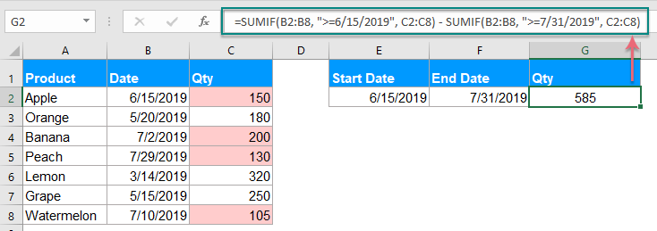
If you want to sum the values if the date between two given dates, you can combine two SUMIF functions together for solving this job.
Please apply the below formula:
And then, press Enter key, the total value between two given dates has been calculated, see screenshot:
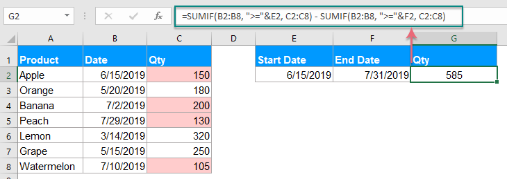
Note: You can also use the cell reference to replace the condition in the above formula as this: =SUMIF(B2:B8, ">="&E2, C2:C8) - SUMIF(B2:B8, ">="&F2, C2:C8), see screenshot:
Example 6: Sum values in multiple columns in Excel
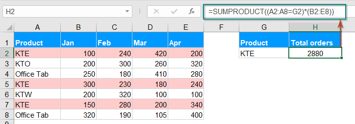
This SUMIF function also can help you to sum values in multiple columns based on one condition. For example, if you have a range of data as below screenshot shown, now, to get the total values of the product KTE in four months - Jan, Feb, Mar and Apr. How could you do?

Normally, the SUMIF function is used to sum a column of values based on one criterion, to sum values in multiple columns, you can combine multiple SUMIF functions for solving this task.
Please apply the below formula into a blank cell:
Then press Enter key to get the correct result you need, see screenshot:

Note: The above SUMIF function is somewhat difficult for you to use if there are a lot of columns need to sum, so here, a simple SUMPRODUCT function can help you deal with this job as well. Please use this formula: =SUMPRODUCT((A2:A8=G2)*(B2:E8)), and then press Enter key to get the result:
- Tips: In the above formula:
- A2:A8: is the range of cells where the criteria will be looking for.
- G2: is the condition you want to sum the cell values based on.
- B2:E8: is the range of cells to be summed.
More SUMIF function articles:
- Sum Corresponding Values With Same Date in Excel
- Have you ever tried to sum corresponding values based on the same date from another column in Excel? Supposing, I have the following data range (A1:B13), column A is the date range contains some duplicate dates, and column B has the number of order, now, I need to add the numbers together based on the same date in column A.How to finish it quickly and easily in Excel?
- Sumif Cells Not Equal To A Specific Value In Excel
- This article, I will talk about how to sum cells if the cells in another column not equal to a specific value in Excel worksheet.
- Sumif Date Is Less/Greater Than Today In Excel
- Supposing we have a sale volume table with planning and actual volumes of every day. Now we are required to count occurred dates before today and calculate the total planning volumes before today in order to dynamically compare the planning volumes and actual volumes. Here I will apply the SUMIF function to get it done in Excel quickly.
- Sumif With One Or More Criteria In Excel
- In Excel, sum values based on one or more criteria is a common task for most of us, the SUMIF function can help us to quickly sum the values based on one condition and the SUMIFS function help us to sum values with multiple criteria. This article, I will describe how to sum with one or more criteria in Excel?
- Sumif Based On Partial Match In Excel
- Take the below data as an example, I want to sum cell values in column B when there contains partial “KTE” text in column A. How to achieve it? This article, I will talk about how to sum cell values based on a partial match in Excel worksheet.
The Best Office Productivity Tools
Kutools for Excel - Helps You To Stand Out From Crowd
Kutools for Excel Boasts Over 300 Features, Ensuring That What You Need is Just A Click Away...
Office Tab - Enable Tabbed Reading and Editing in Microsoft Office (include Excel)
- One second to switch between dozens of open documents!
- Reduce hundreds of mouse clicks for you every day, say goodbye to mouse hand.
- Increases your productivity by 50% when viewing and editing multiple documents.
- Brings Efficient Tabs to Office (include Excel), Just Like Chrome, Edge and Firefox.