Excel VLOOKUP Function
The Excel VLOOKUP function is a powerful tool that helps you look for a specified value by matching on the first column of a table or a range vertically and then return a corresponding value from another column in the same row. Although VLOOKUP is incredibly useful, it can sometimes be challenging to grasp for beginners. This tutorial aims to help you master VLOOKUP by providing step-by-step explanation of the arguments, useful examples and solutions to common errors you may encounter when using the VLOOKUP function.

Related Videos
Step-by-step explanation of arguments
As shown in the above screenshot, the VLOOKUP function is used to find an email based on a given ID number. I will now provide a detailed explanation of how to use VLOOKUP in this example by breaking down each argument step by step.
Step 1: Start the VLOOKUP function
Select a cell (H6 in this case) to output the result, then start the VLOOKUP function by typing the following content in the Formula Bar.
=VLOOKUP(Step 2: Specify the lookup value
First, specify the lookup value (which is what you are looking for) in the VLOOKUP function. Here, I reference cell G6 which contains a certain ID number 1005.
=VLOOKUP(G6
Step 3: Specify the table array
Next, specify a range of cells containing both the value you are looking for and the value you want to return. In this case, I select the range B6:E12. The formula now appears as follows:
=VLOOKUP(G6,B6:E12
=VLOOKUP(G6,$B$6:$E$12Step 4: Specify the column from which you want to return a value
Then specify the column you want to return a value from.
In this example, as I need to return the email based on an ID number, here I enter a number 4 to tell VLOOKUP to return a value from the fourth column of the data range.
=VLOOKUP(G6,B6:E12,4
Step 5: Find an approximate or an exact match
Finally, determine whether you are looking for an approximate match or an exact match.
- To find an exact match, you need to use FALSE as the last argument.
- To find an approximate match, use TRUE as the last argument, or just leave it blank.
In this example, I use FALSE for exact match. The formula now looks like this:
=VLOOKUP(G6,B6:E12,4,FALSE
Press the Enter key to get the result

By explaining each argument one by one in the above example, the syntax and arguments of the VLOOKUP function are now much easier to understand.
Syntax and arguments
=VLOOKUP (lookup_value, table_array, col_index, [range_lookup])
- Lookup_value (required): The value (a real value or a cell reference) you are looking for. Remember this value must be in the first column of the table_array.
- Table_array (required): A range of cells contains both the column of the lookup value and the column of the return value.
- Col_index (required): An integer represents the column number that contains the return value. It starts with number 1 for the left-most column of the table_array.
- Range_lookup (optional): A logical value that determines whether you want VLOOKUP to find an approximate match or an exact match.
- Approximate match - Set this argument to TRUE, 1 or leave it blank.
Important: To find an approximate match, the values in the first column of the table_array must be sorted in ascending order in case VLOOKUP returns the wrong result. - Exact match - Set this argument to FALSE or 0.
- Approximate match - Set this argument to TRUE, 1 or leave it blank.
Examples
This section demonstrates some examples to help you to have a more comprehensive understanding of the VLOOKUP function.
Example 1: Exact match vs. approximate match in VLOOKUP
If you are confused about exact match and approximate match when using VLOOKUP, this section can help you clear up that confusion.
Exact Match in VLOOKUP
In this example, I am going to find the corresponding names based on the scores listed in the range E6:E8, so I enter the following formula in cell F6 and drag the AutoFill handle down to F8. In this formula, the last argument is specified as FALSE to perform an exact match lookup.
=VLOOKUP(E6,$B$6:$C$12,2,FALSE)However, as the score 98 does not exist in the first column of the data range, VLOOKUP returns #N/A error result.

Approximate match in VLOOKUP
Still using the above example, if you change the last argument to TRUE, VLOOKUP will perform an approximate match lookup. If no match is found, it will find the next largest value that is less than the lookup value and return the corresponding result.
=VLOOKUP(E6,$B$6:$C$12,2,TRUE)Since the score 98 does not exist, VLOOKUP finds the next largest value that is less than 98, which is 95, and returns the name of the score 95 as the closest result.

- In this approximate match case, the values in the first column of the table_array must be sorted in ascending order. Otherwise, VLOOKUP may not return the correct value.
- Here I Locked the table array ($B$6:$C$12) in the VLOOKUP function in order to quickly reference a consistent set of data against multiple lookup values.
Example 2: Use VLOOKUP with multiple criteria
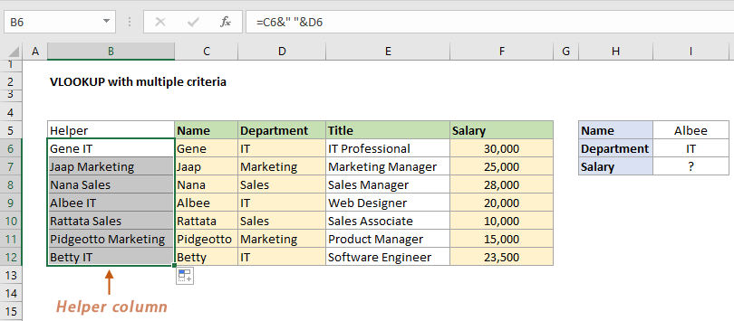
This section demonstrates how to use VLOOKUP with multiple conditions in Excel. As shown in the screenshot below, if you're trying to locate a salary based on a provided name (in cell H5) and department (in cell H6), follow the steps below to get it done.

Step 1: Add a helper column to concatenate the values from the lookup columns
In this case, we need to create a helper column to concatenate the values from the Name column and the Department column.
- Add a helper column to the left of your data range and give a header to this column. See screenshot:

- In this helper column, select the first cell under the header, enter the following formula in the Formula bar, and press Enter.
=C6&" "&D6 Notes: In this formula, we use an ampersand (&) to join the text in two columns to produce a single piece of text.
- C6 is the first name of the Name column to join, D6 is the first department of the Department column to join.
- The values of these two cells are concatenated with a space in between.
- Select this result cell, then drag the AutoFill Handle down to apply this formula to other cells in the same column.


Step 2: Apply the VLOOKUP function with the given criteria
Select a cell where you want to output the result (here I select I7), enter the following formula in the Formula bar, and then press Enter.
=VLOOKUP(I5& " "&I6,B6:F12,5,FALSE)Result

- The helper column must be used as the first column of the data range.
- Now the salary column is the fifth column of the data range, so we use the number 5 as the column index in the formula.
- We need to join the criteria in I5 and I6(I5& " "&I6) the same way as the helper column and use the concatenated value as the lookup_value argument in the formula.
- You also can put the two conditions directly in the lookup_value argument and separate them with a space (if the conditions are text, don’t forget to enclose them in double quotes).
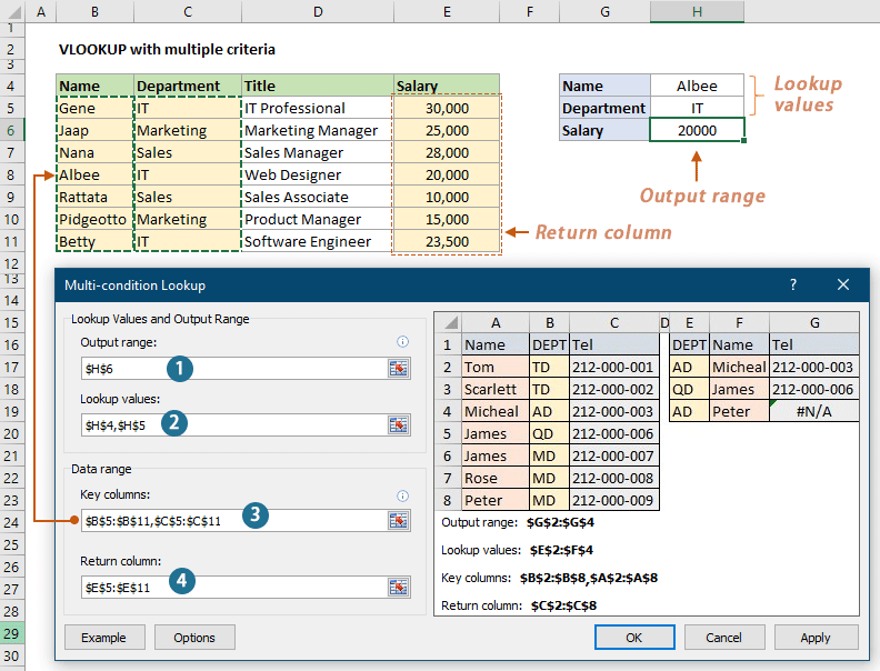
=VLOOKUP("Albee IT",B6:F12,5,FALSE) - A better alternative - lookup with multiple criteria in secondsThe Multi-condition Lookup feature of Kutools for Excel can help you easily lookup with multiple criteria in seconds. Get a 30-day full-featured free trial now!

Common VLOOKUP errors and solutions
This section lists the common errors you may encounter when using VLOOKUP and provides the solutions to fix them.
#N/A error being returned
The most common error with VLOOKUP is the #N/A error, which means that Excel could not find the value you were looking for. Here are some reasons why VLOOKUP may return #N/A error.
Reason 1: The lookup value is not in the first column of the table_array
One of the limitations of Excel VLOOKUP is that it only allows you to look from left to right. So, the lookup values must be in the first column of the table_array.
As shown in the screenshot below, I want to return a name based on the given job title. Here the lookup value (sales manager) is in the second column of the table_array and the return value is to the left of the lookup column, so VLOOKUP returns #N/A error.

Solutions
You can apply any of the following solutions to fix this error.
- Rearrange the columnsYou can rearrange the columns to place the lookup column in the first column of the table_array.
- Use the INDEX and MATCH functions togetherHere we use the INDEX and MATCH functions together as an alternative to VLOOKUP to solve this problem.
=INDEX(B6:B12,MATCH(F6,C6:C12,0))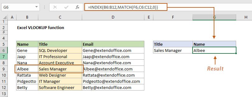
- Use the XLOOKUP function (available in Excel 365, Excel 2021 and later versions)
=XLOOKUP(F6,C6:C12,B6:B12)

Reason 2: The lookup value is not found in the lookup column (exact match)
One of the most common reasons why VLOOKUP returns #N/A error is because the value you are looking for is not found.
As shown in the example below, we are going to find the name based on the given score of 98 in E6. However, this score does not exist in the first column of the data range, so VLOOKUP returns #N/A error result.
Solutions
To fix this error, you can try one of the following solutions.
- If you want VLOOKUP searches for the next largest value that is less than the lookup value, change the last argument FALSE (exact match) to TRUE (approximate match). For more information, please see Example 1: Exact match vs. approximate match using VLOOKUP.
- To avoid changing the last argument and get a reminder in case the lookup value is not found, you can inclose the VLOOKUP function within the IFERROR function:
=IFERROR(VLOOKUP(E8,$B$6:$C$12,2,FALSE),"Not found")
Reason 3: The lookup value is smaller than the smallest value in the lookup column (approximate match)
As shown in the screenshot below, you are performing an approximate match lookup. The value you are looking for (the ID number 1001 in this case) is smaller than the smallest value 1002 in the lookup column, therefore, VLOOKUP returns #N/A error.

Solutions
Here are two solutions for you.
- Ensure that the lookup value is greater than or equal to the smallest value in the lookup column.
- If you want Excel to remind you that the lookup value was not found, just nest the VLOOKUP function in the IFERROR function as follows:
=IFERROR(VLOOKUP(G6,B6:E12,4,TRUE),"Not found")
Reason 4: Numbers are formatted as text
As you can see in the screenshot below, the #N/A error result in this example is due to a data type mismatch between the lookup cell (G6) and the lookup column (B6:B12) of the original table. Here the value in G6 is a number, and the values in the range B6:B12 are numbers formatted as text.

Solutions
To solve this problem, you need to convert the lookup value back to number. Here are two methods for you.
- Apply the Convert to Number featureClick on the cell you want to convert the text to number, select this button
 beside the cell and then select Convert to Number.
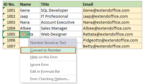
- Apply a handy tool to batch convert between text and numberThe Convert between Text and Number feature of Kutools for Excel helps you easily convert a range of cells from text to number and vice versa. Get a 30-day full-featured free trial now!
 beside the cell and then select Convert to Number.
Reason 5: The table_array is not constant when dragging the VLOOKUP formula to other cells
As shown in the screenshot below, there are two lookup values in E6 and E7. After getting the first result in F6, drag the VLOOKUP formula from cell F6 to F7, an #N/A error result returned. That's because the cell references (B6:C12) are relative by default, and adjusted as you move down through the rows. The table array has been moved down to B7:C13, which no longer contains the lookup score 73.

Solution
You need to lock the table array to keep it constant by adding a $ sign before the rows and columns in the cell references. To know more about absolute reference in Excel, take a look at this tutorial: Excel absolute reference (how to make and use).

#VALUE error being returned
The following conditions may cause VLOOKUP to return #VALUE error result.
Reason 1: The lookup value exceeds 255 characters
As shown in the screenshot below, the lookup value in cell H4 exceeds 255 characters, so VLOOKUP returns a #VALUE error result.

Solutions
To work around this limitation, you can apply a different lookup function that can handle longer strings. Try one of the following formulas.
- INDEX and MATCH:
=INDEX(E5:E11, MATCH(TRUE, INDEX(B5:B11=H4, 0), 0))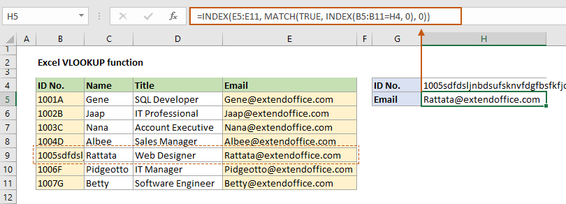
- XLOOKUP function (available in Excel 365, Excel 2021 and later versions):
=XLOOKUP(H4,B5:B11,E5:E11)

Reason 2: The col_index argument is less than 1
The column index specifies the column number in the table array that contains the value you want to return. This argument must be a positive number that corresponds to a valid column in the table array.
If you enter a column index that is less than 1 (i.e., zero or negative), VLOOKUP will not be able to locate the column in the table array.
Solution
To fix this issue, make sure that the column index argument in your VLOOKUP formula is a positive number that corresponds to a valid column in the table array.
#REF error being returned
This section lists one reason why VLOOKUP returns #REF error and provides solutions to this problem.
Reason: The col_index argument is greater than the number of the columns
As you can see in the screenshot below, the table array has only 4 columns. However, the column index you specified in the VLOOKUP formula is 5, which is greater than the number of columns in the table array. As a result, VLOOKUP will not be able to locate the column and will ultimately return a #REF error.

Solutions
- Specify a correct column numberMake sure that the column index argument in your VLOOKUP formula is a number that corresponds to a valid column in the table array.
- Automatically get the column number based on the specified column headerIf the table contains many columns, you may have trouble determining the correct column index number. Here, you can nest the MATCH function in the VLOOKUP function to find the position of the column based on a certian column header.
=VLOOKUP(G6,B6:E12,MATCH("Email",B5:E5,0),FALSE)Note: In the above formula, the MATCH("Email",B5:E5, 0) function is used to get the column number of the "Email" column in the date range B6:E12. Here the result is 4, which is used as the col_index in the VLOOKUP function.
Incorrect value being returned
If you find that VLOOKUP is not returning the correct result, it may be caused by the following reasons
Reason 1: The lookup column is not sorted in ascending order
If you have set the last argument to TRUE (or left it empty) for an approximate match, and the lookup column is not sorted in ascending order, the resulting value may be incorrect.

Solution
Sort the lookup column in ascending order can help you solve this problem. To do this, please follow the below steps:
- Select the data cells in the lookup column, go to the Data tab, click Sort Smallest to Largest in the Sort & Filter group.
- In the Sort Warning dialog box, select the Expand the selection option, and click OK.
Reason 2: A column is inserted or removed
As shown in the screenshot below, the value I originally wanted to return is in the fourth column of the table array, so I specify the col_index number as 4. As a new column is inserted, the result column becomes the fifth column of the table array, causing VLOOKUP to return the result from a wrong column.

Solutions
Here are two solutions for you.
- You can manually change the column index number to match the position of the return column. The formula here should be changed to:
=VLOOKUP(H6,B6:F12,5,FALSE) - If you always want to return the result from a certian column, such as the Email column in this example. The following formula can help to automatically match the column index based on the given column header, regardless of whether columns are inserted or removed from the table array.
=VLOOKUP(H6,B6:F12,MATCH("Email",B5:E5,0),FALSE)
Other function notes
- VLOOKUP only looks for value from left to right.
The lookup value is in the left-most column, and the result value should be in any column to the right of the look up column. - If you leave the last argument blank, VLOOKUP uses approximate match by default.
- VLOOKUP performs a case insensitive lookup.
- For multiple matches, VLOOKUP returns only the first match it finds in the table array, based on the order of the rows in the table array.
Best Office Productivity Tools
Supercharge Your Excel Skills with Kutools for Excel, and Experience Efficiency Like Never Before. Kutools for Excel Offers Over 300 Advanced Features to Boost Productivity and Save Time. Click Here to Get The Feature You Need The Most...
Office Tab Brings Tabbed interface to Office, and Make Your Work Much Easier
- Enable tabbed editing and reading in Word, Excel, PowerPoint, Publisher, Access, Visio and Project.
- Open and create multiple documents in new tabs of the same window, rather than in new windows.
- Increases your productivity by 50%, and reduces hundreds of mouse clicks for you every day!
All Kutools add-ins. One installer
Kutools for Office suite bundles add-ins for Excel, Word, Outlook & PowerPoint plus Office Tab Pro, which is ideal for teams working across Office apps.
- All-in-one suite — Excel, Word, Outlook & PowerPoint add-ins + Office Tab Pro
- One installer, one license — set up in minutes (MSI-ready)
- Works better together — streamlined productivity across Office apps
- 30-day full-featured trial — no registration, no credit card
- Best value — save vs buying individual add-in
Table of contents
- Related Videos
- Step-by-step explanation of arguments
- Syntax and arguments
- VLOOKUP Examples
- Exact match vs. approximate match
- VLOOKUP with multi-conditions
- Common errors and solutions
- #N/A error
- #VALUE error
- #REF error
- Incorrect value
- Other function notes
- Related Articles
- The Best Office Productivity Tools