How to display leader lines in pie chart in Excel?
When you have a large number of data points presented in a pie chart in Excel, the data labels may become crowded and overlap, making it difficult to distinguish and interpret each segment, as shown in the screenshot below. In such situations, displaying leader lines can greatly improve the readability of your pie chart by clearly connecting each data label to its corresponding slice. This enhancement is especially useful for reports, presentations, or dashboards where visual clarity is critical.
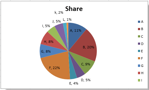
Display leader lines in pie chart
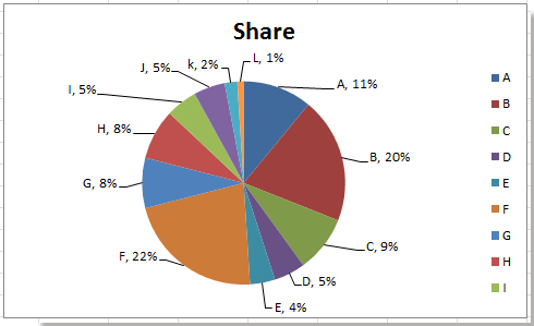
Display leader lines in pie chart
Leader lines in a pie chart are lines that connect each data label to its corresponding slice, helping to prevent confusion when labels are positioned outside the chart. This feature is particularly helpful when:
- Your pie chart contains many similar-sized slices, or data labels are too close together.
- You need to present charts in documents or slides where visual clarity matters.
- The chart will be printed and might lose color distinction between slices.
To display leader lines in your pie chart, you only need to enable a simple option and adjust the labels for better visualization.
1. Click your pie chart in Excel. Then, right-click any data label and choose Format Data Labels from the context menu. If you have trouble right-clicking, make sure you are clicking directly on a data label, not the chart background.

2. In the Format Data Labels pane that appears on the right (or as a dialog box in some Excel versions), locate the Label Options section. Here, check the Show Leader Lines box. If you do not see this option, confirm that you have selected a pie chart and your Excel version supports leader lines.

3. Close the dialog or pane. You should now see leader lines connecting some of your data labels to their respective slices. Note that Excel will only display leader lines for labels positioned outside the pie.

If you want all leader lines to appear (for every slice), click on each data label one by one and drag it outward, away from the pie. Excel will automatically add a leader line for each label moved outside. Be mindful to not drag labels too far—labels that are excessively distant may cause visual clutter. You can use the Undo button (Ctrl+Z) if you move a label accidentally.
If you want to customize the appearance of leader lines, such as changing their color or style for better contrast and emphasis, see this guide: Format leader lines in Excel. Adjusting leader line style can help match them to your chart theme and improve print or digital display.
Common troubleshooting tips: If leader lines do not appear, check that your labels are actually placed outside of the pie. If you still cannot see the "Show Leader Lines" option, confirm your chart type is a standard pie, as this feature is not available for all chart types.
Summary suggestion: Using leader lines in your pie chart improves data readability, especially for charts with many slices and overlapping labels. Remember that dragging labels outside the pie automatically triggers leader lines, and you can format them to match your presentation needs.
Relative Articles:
- Add leader lines to doughnut chart
- Add leader lines to stacked column chart
- Format leader lines in Excel
Best Office Productivity Tools
Supercharge Your Excel Skills with Kutools for Excel, and Experience Efficiency Like Never Before. Kutools for Excel Offers Over 300 Advanced Features to Boost Productivity and Save Time. Click Here to Get The Feature You Need The Most...
Office Tab Brings Tabbed interface to Office, and Make Your Work Much Easier
- Enable tabbed editing and reading in Word, Excel, PowerPoint, Publisher, Access, Visio and Project.
- Open and create multiple documents in new tabs of the same window, rather than in new windows.
- Increases your productivity by 50%, and reduces hundreds of mouse clicks for you every day!
All Kutools add-ins. One installer
Kutools for Office suite bundles add-ins for Excel, Word, Outlook & PowerPoint plus Office Tab Pro, which is ideal for teams working across Office apps.
- All-in-one suite — Excel, Word, Outlook & PowerPoint add-ins + Office Tab Pro
- One installer, one license — set up in minutes (MSI-ready)
- Works better together — streamlined productivity across Office apps
- 30-day full-featured trial — no registration, no credit card
- Best value — save vs buying individual add-in