How to create loan amortization interest calculator of Excel template?
In modern times, it’s quite common to loan money from banks to purchase a house, to pay for tuition, or others. As we know, the loan amortization interest usually is much bigger than we think. You’d better clear with the interest before loaning. This article will show you how to calculate the loan amortization interest in Excel, and then save the workbook as loan amortization interest calculator of Excel template.
Create a loan amortization interest calculation table and save as normal Excel template
 Create loan amortization interest calculator in workbook, and save as an Excel template
Here I will take an example to demonstrate how to calculate the loan amortization interest easily. I loaned $50,000 from a bank, the loan interest rate is 6%, and I plan to repay the loan at the end of every month in coming 10 years.
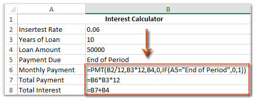
Step 1: Prepare a table, enter the row headers as the following screen shot shown, and input your original data.

Step 2: Calculate the monthly/total payment and total interest with following formulas:

(1) In Cell B6 enter =PMT(B2/12,B3*12,B4,0,IF(A5="End of Period",0,1)), and press the Enter key;
(2) In Cell B7 enter =B6*B3*12, and press the Enter key;
(3) In Cell B8 enter =B7+B4, and press the Enter key.
 | Formula is too complicated to remember? Save the formula as an Auto Text entry for reusing with only one click in future! Read more… Free trial |
Step 3: Format the table as you need.
(1) Select the Range A1:B1, merge this range with clicking Home > Merge & Center, and then add filling color with clicking Home > Fill Color and specify a highlight color.
(2) Then select Range A2:A8, and fill it with clicking Home > Fill Color and specify a highlight color. See screen shot below:

Step 4: Save current workbook as an Excel template:
- In Excel 2013, click the File > Save > Computer > Browse;
- In Excel 2007 and 2010, click the File/Office button > Save.
Step 5: In the coming Save As dialog box, enter a name for this workbook in the File name box, click the Save as type box and select Excel Template (*.xltx) from drop down list, at last click the Save button.

 Related articles:
How to make a read-only template in Excel?
How to protect/lock an Excel template being overwritten with password?
How to find and change default save location of Excel templates?
Best Office Productivity Tools
Supercharge Your Excel Skills with Kutools for Excel, and Experience Efficiency Like Never Before. Kutools for Excel Offers Over 300 Advanced Features to Boost Productivity and Save Time. Click Here to Get The Feature You Need The Most...
Office Tab Brings Tabbed interface to Office, and Make Your Work Much Easier
- Enable tabbed editing and reading in Word, Excel, PowerPoint, Publisher, Access, Visio and Project.
- Open and create multiple documents in new tabs of the same window, rather than in new windows.
- Increases your productivity by 50%, and reduces hundreds of mouse clicks for you every day!
All Kutools add-ins. One installer
Kutools for Office suite bundles add-ins for Excel, Word, Outlook & PowerPoint plus Office Tab Pro, which is ideal for teams working across Office apps.
- All-in-one suite — Excel, Word, Outlook & PowerPoint add-ins + Office Tab Pro
- One installer, one license — set up in minutes (MSI-ready)
- Works better together — streamlined productivity across Office apps
- 30-day full-featured trial — no registration, no credit card
- Best value — save vs buying individual add-in