How to reverse a pivot table in Excel?
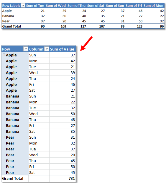
Have you ever wanted to reverse or transpose the pivot table in Excel just like the below screenshots shown. Now I will tell you the quick ways to reverse a pivot table in Excel.
(11 steps) Reverse pivot table with PivotTable and PivotChart Wizard
(7 steps) Reverse pivot table with Kutools for Excel’s Transpose Table Dimensions ![]()
 Reverse pivot table with PivotTable and PivotChart Wizard
To reverse the pivot table, you need to open PivotTable and PivotChart Wizard dialog first and create a new pivot table in Excel.
1. Press Alt + D + P shortcut keys to open PivotTable and PivotChart Wizard dialog, then, check Multiple consolidation ranges option under Where is the data that you want to analyze section and PivotTable option under What kind of report do you want to create section.
Note: You can also add the PivotTabe and PivoChart Wizard command into the Quick Access Toolbar, and click to open the dialog.

2. Click Next to go to the next dialog to check I will create the page fields option, and click the Next.

3. Select your base data, then click Add to add the data range to the All ranges list. See screenshot:

4. Click Next to go to the last step of the Wizard, check the option you need under Where do you want to put the PivotTable report section. Then click Finish.

5. Now a new pivot table is created, and double click last cell at the right down corner of new Pivot table, then a new table is created in a new worksheet. See screenshots:
6. Then create a new pivot table based on this new table. Select the whole new table, and click Insert > PivotTable > PivotTable.

7. Then in the popping dialog, check the option you need under Choose where you want the PivotTable report to be placed section.

8. Click OK. Then a PivotTable Field List pane appears, and drag the Row and Column fields to the Row Labels section, and Value field to Values section. See screenshot:

9. Then click at any cell of the new pivot table, and go to the Design tab to click Report Layout > Show in Tabular Form.

10. Then go to click Report Layout again to click Repeat All Item Labels from the list. See screenshot:

Note: This is no Repeat All Item Labels command in the drop down list of Report Layout button in Excel 2007, just skip this step.
11. Click Design > Subtotals > Do Not Show Subtotals.

Now the pivot table is reversed. See screenshot:

Reverse pivot table with Kutools for Excel’s Transpose Table Dimensions
With above way, there are so many steps to solve the task. To greatly improve your work efficiency and reduce the working hours, I suggest you reverse the pivot table with Kutools for Excel’s Transpose Table Dimensions feature.
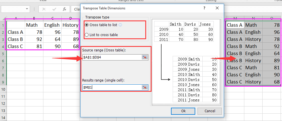
1. Select the base data, and click Kutools > Range > Transpose Table Dimensions.

2. In the Transpose Table Dimensions dialog, check Cross table to list under Transpose type section, then select the cell you want to put the new table.

3. Click Ok to create a new table, and then insert headers above the new table. See screenshot:

4. Select the new table, including the headers, and click Insert > PivotTable > PivotTable, then in the Create PivotTable dialog, check the option you need under Choose where you want the PivotTable report to be placed section.

5. Click OK, and in PivotTable Field List pane, drag Row and Column fields to Row Labels section, and Value field to Values section.
6. Click any cell of the new pivot table and click Design > Report Layout > Show in Tabular Form, then click Report Layout again to click Repeat All Item Labels. See screenshots:
Note: This is no Repeat All Item Labels command in the drop down list of Report Layout button in Excel 2007, just skip it.
7. Click Design > Subtotals > Do Not Show Subtotals.
Now the pivot table is reversed. See screenshot:

With Kutools for Excel’s Transpose Table Dimensions feature, you also can convert list table to cross table. Click here to know more information.
Demo: How To Reverse A Pivot Table In Excel
Quickly transpose Cross table to list or vice versa |
| While you receiving a sheet with cross table which you need to convert to list table, how can you quickly deal with it? With Kutools fro Excel's Transpose Table Dimensions utility, you can convert cross dimensions table to three demensions table or vice versa as quickly as you can. Click for 30-day full-featured free trial! |
 |
| Kutools for Excel: with more than 300 handy Excel add-ins, free to try with no limitation in 30 days. |
Related Articles:
Best Office Productivity Tools
Supercharge Your Excel Skills with Kutools for Excel, and Experience Efficiency Like Never Before. Kutools for Excel Offers Over 300 Advanced Features to Boost Productivity and Save Time. Click Here to Get The Feature You Need The Most...
Office Tab Brings Tabbed interface to Office, and Make Your Work Much Easier
- Enable tabbed editing and reading in Word, Excel, PowerPoint, Publisher, Access, Visio and Project.
- Open and create multiple documents in new tabs of the same window, rather than in new windows.
- Increases your productivity by 50%, and reduces hundreds of mouse clicks for you every day!
All Kutools add-ins. One installer
Kutools for Office suite bundles add-ins for Excel, Word, Outlook & PowerPoint plus Office Tab Pro, which is ideal for teams working across Office apps.
- All-in-one suite — Excel, Word, Outlook & PowerPoint add-ins + Office Tab Pro
- One installer, one license — set up in minutes (MSI-ready)
- Works better together — streamlined productivity across Office apps
- 30-day full-featured trial — no registration, no credit card
- Best value — save vs buying individual add-in