
How to lookup a value and return cell address in Excel?

In general, you will get the cell value when you use formula to look up a value in Excel. But here I will introduce some formulas to lookup a value and return the relative cell address.

Lookup a value and return cell address with formula


arrow blue right bubble Lookup a value and return cell address with formula

To lookup a value and return corresponding cell address instead of cell value in Excel, you can use the below formulas.

Formula 1 To return the cell absolute reference

For example, you have a range of data as below screenshot shown, and you want to lookup product AA and return the relative cell absolute reference.
doc-vlookup-return-cell-address-1

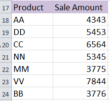
1. Select a cell and type AA into it, here I type AA into cell A26. See screenshot:
doc-vlookup-return-cell-address-2

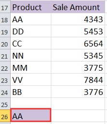
2. Then type this formula =CELL("address",INDEX($A$18:$A$24,MATCH(A26,$A$18:$A$24,1))) in the cell adjacent to cell A26 (the cell you typed AA), then press Shift + Ctrl + Enter keys and you will get the relative cell reference. See screenshot:
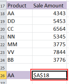
doc-vlookup-return-cell-address-3

Tip:

1. In the above formula, A18:A24 is the column range that your lookup value is in, A26 is the lookup value.

2. This formula only can find the first relative cell address which matches the lookup value.

Formula 2 To return the row number of the cell value in the table

For instance, you have data as below screenshot shown, you want to lookup product BB and return all of its cell addresses in the table.
doc-vlookup-return-cell-address-4

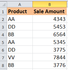
1. Type BB into a cell, here I type BB into cell A10. See screenshot:
doc-vlookup-return-cell-address-5

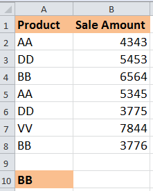
2. In the cell adjacent to the cell A10 (the cell you typed BB), type this formula =SMALL(IF($A$10=$A$2:$A$8, ROW($A$2:$A$8)-ROW($A$2)+1), ROW(1:1)), and press Shift + Ctrl + Enter keys, then drag the auto fill handle down to apply this formula until appears #NUM!. see screenshot:
doc-vlookup-return-cell-address-6

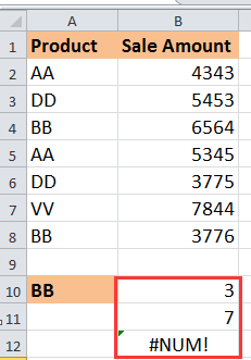
3. Then you can delete #NUM!. See screenshot:
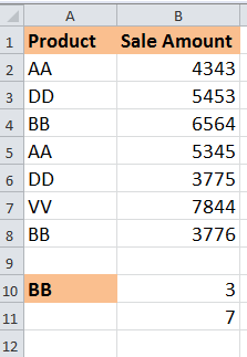
doc-vlookup-return-cell-address-7

Tips:

1. In this formula, A10 indicates the lookup value, and A2: A8 is the column range that your lookup value is in.

2. With this formula, you only can get the row numbers of the relative cells in the table except table header.

Batch Convert formula reference to absolute, relative, column absolute or Row Absolute

Sometimes, you may want to convert the formula reference to absolute, but in Excel, the shortcuts only can convert the references one by one whihc may waste time while there are hundreds of formulas. The Convert Reference of Kutools for Excel can batch convert the references in select cells to relative, absolute as you need.   Click for full-featured 30 days free trial!
doc kutools convert reference 1
 
Kutools for Excel: with more than 300 handy Excel add-ins, free to try with no limitation in 30 days.

Relative Articles

Best Office Productivity Tools

🤖 Kutools AI Aide: Revolutionize data analysis based on: Intelligent Execution   |  Generate Code  |  Create Custom Formulas  |  Analyze Data and Generate Charts  |  Invoke Kutools Functions
Popular Features: Find, Highlight or Identify Duplicates   |  Delete Blank Rows   |  Combine Columns or Cells without Losing Data   |   Round without Formula ...
Super Lookup: Multiple Criteria VLookup    Multiple Value VLookup  |   VLookup Across Multiple Sheets   |   Fuzzy Lookup ....
Advanced Drop-down List: Quickly Create Drop Down List   |  Dependent Drop Down List   |  Multi-select Drop Down List ....
Column Manager: Add a Specific Number of Columns  |  Move Columns  |  Toggle Visibility Status of Hidden Columns  |  Compare Ranges & Columns ...
Featured Features: Grid Focus   |  Design View   |   Big Formula Bar    Workbook & Sheet Manager   |  Resource Library (Auto Text)   |  Date Picker   |  Combine Worksheets   |  Encrypt/Decrypt Cells    Send Emails by List   |  Super Filter   |   Special Filter (filter bold/italic/strikethrough...) ...
Top 15 Toolsets12 Text Tools (Add Text, Remove Characters, ...)   |   50+ Chart Types (Gantt Chart, ...)   |   40+ Practical Formulas (Calculate age based on birthday, ...)   |   19 Insertion Tools (Insert QR Code, Insert Picture from Path, ...)   |   12 Conversion Tools (Numbers to Words, Currency Conversion, ...)   |   7 Merge & Split Tools (Advanced Combine Rows, Split Cells, ...)   |   ... and more

Supercharge Your Excel Skills with Kutools for Excel, and Experience Efficiency Like Never Before. Kutools for Excel Offers Over 300 Advanced Features to Boost Productivity and Save Time.  Click Here to Get The Feature You Need The Most...

Description


Office Tab Brings Tabbed interface to Office, and Make Your Work Much Easier

  • Enable tabbed editing and reading in Word, Excel, PowerPoint, Publisher, Access, Visio and Project.
  • Open and create multiple documents in new tabs of the same window, rather than in new windows.
  • Increases your productivity by 50%, and reduces hundreds of mouse clicks for you every day!
Comments (26)
No ratings yet. Be the first to rate!
This comment was minimized by the moderator on the site
HI. In sheet 1, I need a certain value present in sheet 2 to be returned. Therefore, in column A of sheet 2, first of all I have to look for a cell containing a specific text (all the cells in column A contain a different text) . From this cell I have to go two rows down and 33 columns to the right of this specific text cell. This is the sheet 2 cell containing my value to import into sheet 1. How can I do this? Could you please help me ? Thank you very much
This comment was minimized by the moderator on the site
Die Formel =CELL("address",INDEX($A$18:$A$24,MATCH(A26,$A$18:$A$24,1))) ist genau das, was ich suche!!!

Tipp 2. "Diese Formel kann nur die erste relative Zellenadresse finden, die dem Suchwert entspricht." beschreibt genau mein Problem: ich benötige die letzte relative Zellenadresse, die dem Suchwert entspricht. Ist das machbar?

Danke und Gruß
Micha
This comment was minimized by the moderator on the site
Hi, Damich, below formula will lookup value from bottom, and return the relative cell address:
=CELL("address",INDEX($A$1:$A$7,MATCH(2,1/($A$1:$A$7=A10),1)))
This comment was minimized by the moderator on the site
If my data is in any sheet of the workbook whether in sheet 1, or sheet 2, or sheet 3, how can I find the cell address of this data with the help of formula.

pls advise.....
This comment was minimized by the moderator on the site
Hi, you can add the sheet name in the formula: =CELL("address",INDEX(Sheet1!$A$18:$A$24,MATCH(A26,Sheet1!$A$18:$A$24,1))), Sheet1 is the sheet name that contains your data.
This comment was minimized by the moderator on the site
감사합니다.

다만
=CELL("address",INDEX($A$18:$A$24,MATCH(A26,$A$18:$A$24,1)))
->
=CELL("address",INDEX($A$18:$A$24,MATCH(A26,$A$18:$A$24,0)))
MATCH함수 마지막에 1이 아닌 0을 기입해야
AA가 아닌 BB의 위치도 반환이 되는 것 같아요.

훌륭한 설명 감사합니다.

큰 도움이 됬어요.
This comment was minimized by the moderator on the site
Is there any formula for this case below to summarize following Alphabet of results? For example: which numbers belong to A/B/..
A=1; E=42; D=64; C=32; B=20; D=9; A=10; B=22; D=45; C=21; E=30; E=59; A=33; D=23; C=11; B=25; B=49; D=6; D=99; E=89; A=70; D=27; B=4; C=47; D=68; E=62; A=57; A=86; B=91; D=93; C=18; D=12; A=55; D=50; ect.
==> expect for result: A=1;10;33;70;57;86;55
My email: thanks so much
This comment was minimized by the moderator on the site
Can we modify the formula =CELL("address",INDEX($A$18:$A$24,MATCH(A26,$A$18:$A$24,1))) to get all the cell addresses which contains a specific text string like an array formula
This comment was minimized by the moderator on the site
Can we modify the formula =CELL("address",INDEX($A$18:$A$24,MATCH(A26,$A$18:$A$24,1))) to get all the cell addresses which contains a specific text string
This comment was minimized by the moderator on the site
Have no idea.
This comment was minimized by the moderator on the site
=CELL("address",INDEX($A$18:$A$24,MATCH(A26,$A$18:$A$24,1))) excellent this function for me but i want cell reference address across multiple sheets.
This comment was minimized by the moderator on the site
Try to add the sheet name in the formula like =CELL("address",INDEX(Sheet1!$A$18:$A$24,MATCH(Sheet2!A26,Sheet1!$A$18:$A$24,1))).
This comment was minimized by the moderator on the site
I would like to lookup the address of the max value in column.
This comment was minimized by the moderator on the site
Hi, sorry to repy so late, if you also need the answer, this tutorial will help you: How To Find Address Of Cell With Max Or Min Value In Excel?
This comment was minimized by the moderator on the site
Hi Master,

What formula for search "value" belong to which sheet , address in excel file with 100 worksheet tab
There are no comments posted here yet
Load More
Please leave your comments in English
Posting as Guest
×
Rate this post:
0   Characters
Suggested Locations