How to vlookup value and return true or false / yes or no in Excel?
In many cases, you may need to look for values in a column and just return true or false (yes or no) if the value was found or not in another column. In this article, we are going to show you methods to achieve it.
Vlookupand return true or false / yes or no with formula
Highlight values in a column if they are found in another column with an amazing tool
More tutorials for VLOOKUP...
Vlookupand return true or false / yes or no with formula
Supposing you have a list of data in range A2:A18 as shown in following screenshot. To search the values in A2:A18 according to the value in D2:D4 and display the result True or false / Yes or No, please do as follows.

1. Select a blank cell to output the result. Here I select B2.
2. Enter the below formula into it and press the Enter key.
=IF(ISNA(VLOOKUP(A2,$D$2:$D$4,1,FALSE)), "No", "Yes")
3. Select the result cell, and then drag the Fill Handle to apply the formula to other cells (In this case, I drag the Fill Handle down until it reaches B18). See screenshot:

Note: For returning True or False, please replace the “Yes” and “No” in the formula with “True” and “False”:
=IF(ISNA(VLOOKUP(A2,$D$2:$D$4,1,FALSE)), "False", "True")

Highlight values in a column if they are found in another column with an amazing tool
If you want to stand out values (such as highlight them with background color) in a column if they are found in another column, here highly recommended the Select Same & Different Cells utility of Kutools for Excel. With this utility, you can easily achieve it by clicks only. as the below demo shown. Download Kutools for Excel now! (30-day free trail)
Let's see how to apply this feature to highlight values in a column if they are found in another column.
1. After installing Kutools for Excel, click Kutools > Select > Select Same & Different Cells to enable the utility.

2. In the Select Same & Different Cells dialog box, please configure as follows.
- 2.1) In the Find values in box, select the range which you will highlight values in;
- 2.2) In the According to box, select the range you will highlight values based on;
- 2.3) In the Based on section, check the Single cell option;
- 2.4) In the Find section, choose the Same values option;
- 2.5) In the Processing of results section, check the Fill backcolor or Fill font color as you need, specify a highlight color;
- 2.6) Click the OK button. See screenshot:

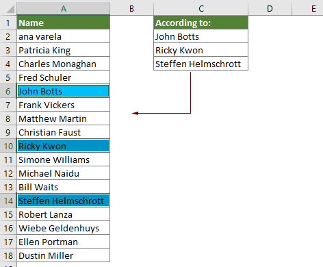
Then, if values in range A2:A18 was found in C2:C4, they will be highlighted and selected immediately as the below screenshot shown.

If you want to have a free trial (30-day) of this utility, please click to download it, and then go to apply the operation according above steps.
related articles
Vlookup values across multiple worksheets
You can apply the vlookup function to return the matching values in a table of a worksheet. However, if you need to vlookup value across multiple worksheets, how can you do? This article provides detailed steps to help you easily solve the problem.
Vlookup and return matched values in multiple columns
Normally, applying the Vlookup function can only return the matched value from one column. Sometimes, you may need to extract matched values from multiple columns based on the criteria. Here is the solution for you.
Vlookup to return multiple values in one cell
Normally, when applying the VLOOKUP function, if there are multiple values that match the criteria, you can only get the result of the first one. If you want to return all matched results and display them all in a single cell, how can you achieve?
Vlookup and return entire row of a matched value
Normally, using the vlookup function can only return a result from a certain column in the same row. This article is going to show you how to return the whole row of data based on specific criteria.
Backwards Vlookup or in reverse order
In general, the VLOOKUP function searches values from left to right in the array table, and it requires the lookup value must stay in the left side of target value. But, sometimes you may know the target value and want to find out the lookup value in reverse. Therefore, you need to vlookup backwards in Excel. There are several ways in this article to deal with this problem easily!
Best Office Productivity Tools
Supercharge Your Excel Skills with Kutools for Excel, and Experience Efficiency Like Never Before. Kutools for Excel Offers Over 300 Advanced Features to Boost Productivity and Save Time. Click Here to Get The Feature You Need The Most...
Office Tab Brings Tabbed interface to Office, and Make Your Work Much Easier
- Enable tabbed editing and reading in Word, Excel, PowerPoint, Publisher, Access, Visio and Project.
- Open and create multiple documents in new tabs of the same window, rather than in new windows.
- Increases your productivity by 50%, and reduces hundreds of mouse clicks for you every day!
All Kutools add-ins. One installer
Kutools for Office suite bundles add-ins for Excel, Word, Outlook & PowerPoint plus Office Tab Pro, which is ideal for teams working across Office apps.
- All-in-one suite — Excel, Word, Outlook & PowerPoint add-ins + Office Tab Pro
- One installer, one license — set up in minutes (MSI-ready)
- Works better together — streamlined productivity across Office apps
- 30-day full-featured trial — no registration, no credit card
- Best value — save vs buying individual add-in
