Find the last occurrence of a Lookup value in Excel (Optimized Guide)
By default, Excel's VLOOKUP function returns the first matching result when searching for a value. However, if your list contains multiple matching values and you need to return the last occurrence, how can you achieve this? This article explores multiple optimized methods to find the last match of a lookup value in a list—suitable for both basic and advanced Excel users.
Find the last occurrence of a Lookup value in Excel
Find the last occurrence of a Lookup value with INDEX and MATCH functions
This method works in all Excel versions and is based on a combination of INDEX and MATCH array formula.
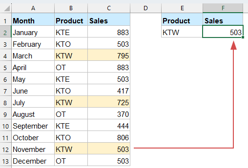
=INDEX($C$2:$C$13,MATCH(2,1/(B2:B13=E2)))
- B2:B13=E2: Checks which cells in range B2:B13 match the product in E2.
- 1/(B2:B13=E2): Converts TRUE to 1 and FALSE to #DIV/0! (division error).
- MATCH(2, 1/(B2:B13=E2)):
o Searches for the number 2 in the array.
o Since 2 doesn’t exist, MATCH returns the position of the last numeric value (1).
o This gives the row number of the last "KTW" in column B. - INDEX($C$2:$C$13, ...): Returns the sales value from column C at the row found by MATCH.
Find the last occurrence of a Lookup value with Kutools for Excel
If you frequently work with advanced lookups, Kutools for Excel offers a powerful, point-and-click solution that allows you to perform complex data retrieval tasks effortlessly—without the need to write or memorize complex formulas.
This makes it especially valuable for users who handle large datasets regularly or who prefer a more visual, user-friendly interface over traditional formula-based methods. Whether you're a beginner or an experienced Excel user, Kutools can help streamline your workflow and significantly improve productivity.
After installing Kutools for Excel, please do with the following steps:
1. Click Kutools > Super LOOKUP > LOOKUP from Bottom to Top to enable the feature. See screenshot:

2. In the LOOKUP from Bottom to Top dialog box, please configure as follows.
- Select the lookup value cells and the output cells in the Lookup Values and Output Range section;
- Select the whole data range, the key column you are looking for, and the return column in the Data range section;
- Click the OK button to get the results immediately. See screenshot:

Find the last occurrence of a Lookup value with XLOOKUP function
With Excel 365 or Excel 2021, you can simplify the process using XLOOKUP, which natively supports reverse searches.
Enter the following formula into a blank cell, and press Enter key to get the last corresponding value as follows:
=XLOOKUP(E2, $B$2:$B$13, $C$2:$C$13,,,-1)
- E2 is the value you want to find.
- $B$2:$B$13 is the range where you search for the value.
- $C$2:$C$13 is the range from which to return the result.
- The last argument -1 tells Excel to search from the bottom up, so it finds the last match.
📝 Conclusion
Finding the last occurrence of a lookup value in Excel can be achieved in several effective ways, depending on your version of Excel and personal preference.
- The INDEX and MATCH method is reliable and works in all versions, though it requires array logic.
- The XLOOKUP function, available in Excel 365 and 2021, provides a cleaner and more intuitive solution with built-in support for reverse searching.
- For users who prefer a no-code approach, Kutools for Excel offers a user-friendly interface that handles advanced lookups with just a few clicks.
No matter which method you choose, each can help you quickly retrieve the latest relevant data and enhance your data analysis efficiency. If you're interested in exploring more Excel tips and tricks, our website offers thousands of tutorials to help you master Excel.
Related articles
Find earliest and latest dates in a range in Excel
In a column of dates, it's not easy to find out the earliest date and latest date quickly if you can't sort the dates. Actually, there are several tricky ways to find out the earliest and latest dates in Excel easily and conveniently, you can follow the methods in this article to get it down.
Find or get quarter from a given date in Excel
Supposing you have a list of dates in a column, and now you want to find and get the quarters from these dates, how can you quickly handle it in Excel? This article is going to introduce the tricks on deal with this job.
Vlookup to compare two lists in separated worksheets
Supposing you have two worksheets “Name-1” and “Name-2” with a list of names, and now you want to compare these two lists and find the matching names in Names-1 if they exit in Names-2. It is painful to do such a comparison manually one by one between two sheet. This article is provides some quick tricks to help you to finish it without effort.
Vlookup and sum matches in rows or columns in Excel
Using vlookup and sum function helps you quickly find out the specified criteria and sum the corresponding values at the same time. In this article, we are going to show you two methods to vlookup and sum the first or all matched values in rows or columns in Excel.
Best Office Productivity Tools
Supercharge Your Excel Skills with Kutools for Excel, and Experience Efficiency Like Never Before. Kutools for Excel Offers Over 300 Advanced Features to Boost Productivity and Save Time. Click Here to Get The Feature You Need The Most...
Office Tab Brings Tabbed interface to Office, and Make Your Work Much Easier
- Enable tabbed editing and reading in Word, Excel, PowerPoint, Publisher, Access, Visio and Project.
- Open and create multiple documents in new tabs of the same window, rather than in new windows.
- Increases your productivity by 50%, and reduces hundreds of mouse clicks for you every day!
All Kutools add-ins. One installer
Kutools for Office suite bundles add-ins for Excel, Word, Outlook & PowerPoint plus Office Tab Pro, which is ideal for teams working across Office apps.
- All-in-one suite — Excel, Word, Outlook & PowerPoint add-ins + Office Tab Pro
- One installer, one license — set up in minutes (MSI-ready)
- Works better together — streamlined productivity across Office apps
- 30-day full-featured trial — no registration, no credit card
- Best value — save vs buying individual add-in