Split cells in Excel (full guide with detailed steps)
In Excel, there are various reasons why you might need to split cell data. For example, the raw data may contain multiple pieces of information lumped into one cell, such as full names or addresses. Splitting these cells allows you to separate different types of information, making the data easier to clean and analyze. This article will serve as your comprehensive guide, showing different ways to split cells into rows or columns based on specific separators.

Split cells in Excel into multiple columns
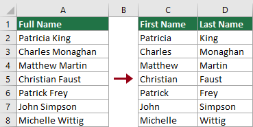
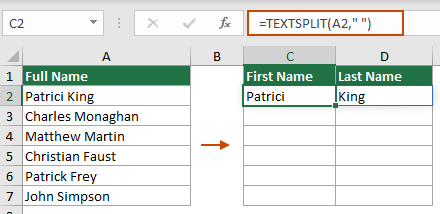
As shown in the following screenshot, suppose you have a list of full names, and you want to split each full name into separate first and last names and place the split data in separate columns. This section will demonstrate four ways to help you accomplish this task.
Split cells into multiple columns with Text to Column wizard
To split cells into multiple columns based on a specific separator, one commonly used method is the Text to Column wizard in Excel. Here, I will show you step-by-step how to use this wizard to achieve the desired result.
Step 1: Select the cells you wish to split and open the Text to Columns wizard
In this case, I select the range A2:A8, which contains full names. Then go to the Data tab, click Text to Columns to open the Text to Columns wizard.

Step 2: Configure the steps one by one in the wizard
- In the Step 1 of 3 wizard, select the Delimited option and then click the Next button.

- In the Step 2 of 3 wizard, select the delimiters for your data and then click the Next button to continue.In this case, since I need to split full names into first and last names based on spaces, I only select the Space checkbox in the Delimiters section.
 Notes:
- If the delimiter you need is not shown in this section, you can select the Other checkbox and enter your own delimiter into the textbox.
- To split cells by line break, you can select the Other checkbox and press Ctrl + J keys together.

- In the last wizard, you need to configure as follows:1) In the Destination box, select a cell to place the split data. Here I choose cell C2.2) Click the Finish button.


Result
Full names in selected cells are separated into first and last names and located in different columns.
Conveniently split cells into multiple columns using Kutools
As you can see, the Text to Columns wizard requires multiple steps to complete the task. If you need a simpler method, the Split Cells feature of Kutools for Excel is highly recommended. With this feature, you can conveniently split cells into multiple columns or rows based on a specific delimiter, by completing the settings in a single dialog box.
After installing Kutools for Excel, select Kutools > Merge & Split > Split Cells to open the Split Cells dialog box.
- Select the range of cells containing the text you wish to split.
- Select the Split to Columns option.
- Select Space (or any delimiter you need) and click OK.

- Select a destination cell and click OK to get all split data.
Split cells into multiple columns with Flash Fill
Now let’s move on to the third method, known as Flash Fill. Introduced in Excel 2013, Flash Fill designed to automatically fill your data when it senses a pattern. In this section, I will demonstrate how to use the Flash Fill feature to separate first and last names from full names in a single column.
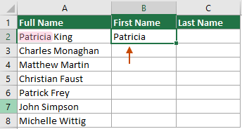
Step 1: Manually enter the first split data in the cell adjacent to the original column
In this case, I am going to split the full names in column A into separate first and last names. The first full name is in cell A2, so I select the cell B2 adjacent to it and type the first name. See screenshot:
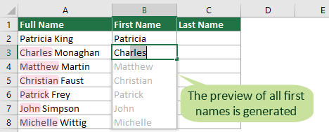
Step 2: Apply the Flash Fill to automatically fill all first names
Start typing the second first name into the cell below B2 (which is B3), then Excel will recognize the pattern and generate a preview of the rest of the first names, and you need to press Enter to accept the preview.
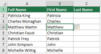
Now all first names of full names in column A are separated in column B.
Step 3: Get last names of full names in another column
You need to repeat the above Steps 1 and 2 to split the last names from the full names in Column A into the column next to the first name column.
Result

- This feature is only available in Excel 2013 and later versions.
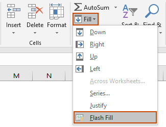
- You can also access the Flash Fill with one of the following methods.
- By shortcutAfter typing the first name in cell B2, select the range B2:B8, press Ctrl + E keys to automatically fill the rest of the first names

- By ribbon optionAfter typing the first name in cell B2, select the range B2:B8, go to click Fill > Flash Fill under the Home tab.
- By shortcut
Split cells into multiple columns with formulas
The above methods are not dynamic, which means if the source data changes, then we need to rerun the same process over again. Take the same example as above, to split the full names listing in Column A into separate first and last names and have the split data update automatically with any changes in the source data, please try one of the following formulas
Use TEXT functions to split cells into columns by certain delimiter
The formulas provided in this section are available in all Excel versions. To apply the formulas, do as follows.
Step 1: Extract the text before the first delimiter (first names in this case)
- Select a cell (C2 in this case) to output the first name, enter the following formula and press Enter to get the first name in A2.
=LEFT(A2,SEARCH(" ",A2)-1)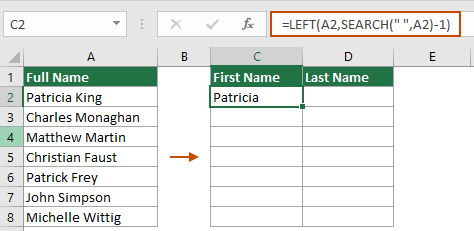
- Select this result cell and drag its AutoFill Handle down to get the rest of the first names.


Step 2: Extract the text after the first delimiter (last names in this case)
- Select a cell (D2 in this case) to output the last name, enter the following formula and press Enter to get the last name in A2.
=RIGHT(A2,LEN(A2)-SEARCH(" ",A2))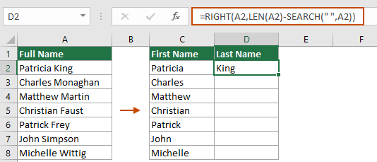
- Select this result cell and drag its AutoFill Handle down to get the rest of the last names.


- In the above formulas:
- A2 is the cell containing the full name I wish to split.
- A space in quotation marks indicates that the cell will be split by a space. You can change the reference cell and the delimiter according to your needs.
- If a cell contains more than two texts divided by spaces that need to be split, the second formula provided above will return incorrect result. You will need additional formulas to correctly split the second, third, and up to the Nth value separated by spaces.
- Use the following formula to return the second word (e.g., middle name) separated by spaces.
=TRIM(MID(SUBSTITUTE(A2," ",REPT(" ", 100)),100,100))
- Change the second 100 to 200 to get the third word (e.g., last name) separated by spaces.
=TRIM(MID(SUBSTITUTE(A2," ",REPT(" ", 100)),200,100))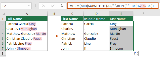
- By changing 200 to 300, 400, 500, etc., you can obtain the fourth, fifth, sixth, and subsequent words.
- Use the following formula to return the second word (e.g., middle name) separated by spaces.


Use the TEXTSPLIT function to split cells into columns by specific separator
If you are using Excel for Microsoft 365, the TEXTSPLIT function is more recommended. Please do as follows.
Step 1: Select a cell to output the result. Here I select the cell C2
Step 2: Enter the below formula and press Enter
=TEXTSPLIT(A2," ")You can see that all the text separated by spaces in A2 is split into different columns.
Step 3: Drag the formula to get all results
Select the result cells in the same row, then drag the AutoFill Handle down to get all results.
- This function is only available in Excel for Microsoft 365.
- In this formula
- A2 is the cell containing the full name I wish to split.
- A space in quotation marks indicates that the cell will be split by a space. You can change the reference cell and the delimiter according to your needs.
Split cells in Excel into multiple rows
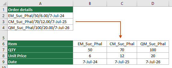
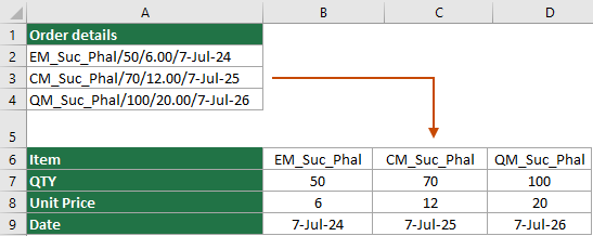
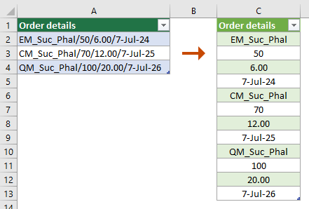
As shown in the screenshot below, there is a list of order details in the range A2:A4, and the data needs to be split using a slash to extract different types of information such as Item, Quantity, Unit Price and Date. To accomplish this task, this section demonstrates 3 methods.
Split cells into multiple rows with TEXTSPLIT function
If you are using Excel for Microsoft 365, the TEXTSPLIT function method can easily help. Please do as follows.
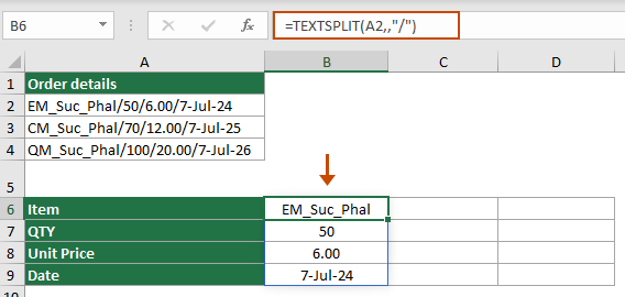
Step 1: Select a cell to output the result. Here I select the cell B6
Step 2: Type the below formula and press Enter
=TEXTSPLIT(A2,,"/")All text in A2 is split into separate rows based on the 'slash' separator.
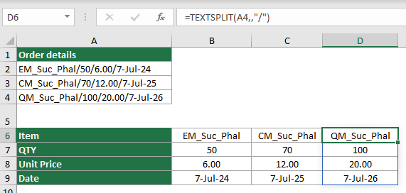
To split data in cells A3 and A4 into individual rows based on slashes, simply repeat steps 1 and 2 with the appropriate formulas below.
Formula in C6:
=TEXTSPLIT(A3,,"/")Formula in D6:
=TEXTSPLIT(A4,,"/")Result
- This function is only available in Excel for Microsoft 365.
- In the above formulas, you can change the slash / in the quotation marks to any delimiter according to your data.
Conveniently split cells into multiple rows using Kutools
Although Excel's TEXTSPLIT feature is very useful, it is limited to Excel for Microsoft 365 users. Moreover, if you have multiple cells in a column to split, you will need to apply different formulas individually to each cell to get the results. In contrast, Kutools for Excel's Split Cells feature is working across all Excel versions. It provides a straightforward, efficient solution to split cells into multiple rows or columns at once with just a few clicks.
After installing Kutools for Excel, click Kutools > Merge & Split > Split Cells to open the Split Cells dialog box.
- Select the range of cells containing the text you wish to split.
- Select the Split to Rows option.
- Select a delimiter you need (here I select the Other option and enter a slash), then click OK.
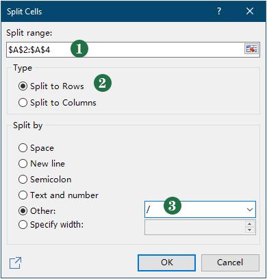
- Select a destination cell and click OK to get all split data
Split cells into multiple rows with VBA code
This section provides a VBA code for you to easily split cells into multiple rows in Excel. Please do as follows.
Step 1: Open the Microsoft Visual Basic for Applications window
Press the Alt + F11 keys to open this window.
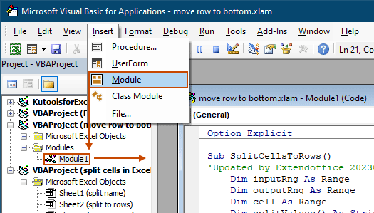
Step 2: Insert a module and enter VBA code
Click Insert > Module, and then copy and paste the following VBA code into the Module (Code) window.
VBA code: Split cells into multiple rows in Excel
Option Explicit

Sub SplitCellsToRows()
'Updated by Extendoffice 20230727
    Dim inputRng As Range
    Dim outputRng As Range
    Dim cell As Range
    Dim splitValues() As String
    Dim delimiter As String
    Dim i As Long
    Dim columnOffset As Long
    On Error Resume Next

    Set inputRng = Application.InputBox("Please select the input range", "Kutools for Excel", Type:=8) ' Ask user to select input range
    If inputRng Is Nothing Then Exit Sub ' If the user clicked Cancel or entered nothing, exit the sub
    Set outputRng = Application.InputBox("Please select the output range", "Kutools for Excel", Type:=8) ' Ask user to select output range
    If outputRng Is Nothing Then Exit Sub ' If the user clicked Cancel or entered nothing, exit the sub
    delimiter = Application.InputBox("Please enter the delimiter to split the cell contents", "Kutools for Excel", Type:=2) ' Ask user for delimiter
    If delimiter = "" Then Exit Sub ' If the user clicked Cancel or entered nothing, exit the sub
    If delimiter = "" Or delimiter = "False" Then Exit Sub ' If the user clicked Cancel or entered nothing, exit the sub

    Application.ScreenUpdating = False

    columnOffset = 0
    For Each cell In inputRng
        If InStr(cell.Value, delimiter) > 0 Then
            splitValues = Split(cell.Value, delimiter)
            For i = LBound(splitValues) To UBound(splitValues)
                outputRng.Offset(i, columnOffset).Value = splitValues(i)
            Next i
            columnOffset = columnOffset + 1
        Else
            outputRng.Offset(0, columnOffset).Value = cell.Value
            columnOffset = columnOffset + 1
        End If
    Next cell

    Application.ScreenUpdating = True
End Sub
Step 3: Run the VBA code
Press the F5 key to run the code. Then you need to do the following configurations.
- A dialog box will appear prompting you to select the cells with the data you want to split (here I select the range A2:A4). After making your selection, click OK.

- In the second popping up dialog box, you need to select the output range (here I select the cell B6), and then click OK.

- In the last dialog box, enter the delimiter used to split the cell contents (here I enter a slash) and then click the OK button.


Result
Cells in the selected range are split into multiple rows at the same time.
Split cells into multiple rows with Power Query
Another method for splitting cells into multiple rows by certain delimiter is to use Power Query, which can also make the split data dynamically change with the source data. The downside to this method is that it takes multiple steps to complete. Let's dive in to see how it works.
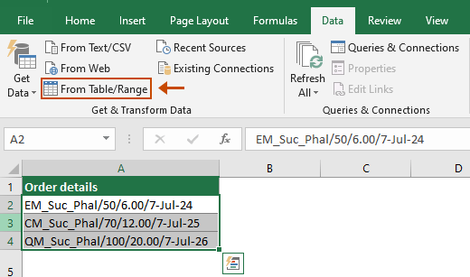
Step 1: Select the cells you want to split into multiple rows, select Data > From Table / Range
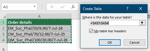
Step 2: Convert the selected cells to table
If the selected cells are not Excel table format, a Create Table dialog box will pop up. In this dialog box, you just need to verify if Excel has picked your selected cell range correctly, mark if your table has header, and then click the OK button.
If the selected cells are Excel table, jump to Step 3.
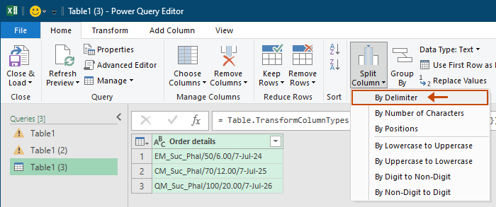
Step 3: Choose Split Column By Delimiter
A Table – Power Query Editor window pops up, click Split Column > By Delimiter under the Home tab.
Step 4: Configure the Split Column by Delimiter dialog box
- In the Select or enter the delimiter section, specify a delimiter for splitting the text (Here I choose Custom and enter a slash / in the textbox).
- Expand the Advanced Options section (which is folded by default) and select the Rows option.
- In the Quote Character section, choose None from the drop-down list;
- Click OK.


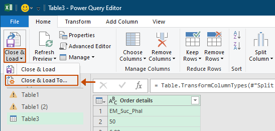
Step 5: Save and load the split data
- In this case, as I need to specify a custom destination for my split data, I click Close & Load > Close & Load To.
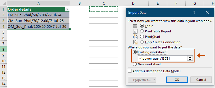
 Tip: To load the split data in a new worksheet, choose the Close & Load option.
 - In the Import Data dialog box, choose the Existing worksheet option, select a cell to locate the split data, and then click OK.


Result
Then all cells in the selected range are split into different rows within the same column by specified delimiter.
In conclusion, this article has explored different methods to split cells into multiple columns or rows in Excel. No matter which approach you choose, mastering these techniques can greatly enhance your efficiency when dealing with data in Excel. Keep exploring, and you'll find the method that works best for you.
Best Office Productivity Tools
Supercharge Your Excel Skills with Kutools for Excel, and Experience Efficiency Like Never Before. Kutools for Excel Offers Over 300 Advanced Features to Boost Productivity and Save Time. Click Here to Get The Feature You Need The Most...
Office Tab Brings Tabbed interface to Office, and Make Your Work Much Easier
- Enable tabbed editing and reading in Word, Excel, PowerPoint, Publisher, Access, Visio and Project.
- Open and create multiple documents in new tabs of the same window, rather than in new windows.
- Increases your productivity by 50%, and reduces hundreds of mouse clicks for you every day!
All Kutools add-ins. One installer
Kutools for Office suite bundles add-ins for Excel, Word, Outlook & PowerPoint plus Office Tab Pro, which is ideal for teams working across Office apps.
- All-in-one suite — Excel, Word, Outlook & PowerPoint add-ins + Office Tab Pro
- One installer, one license — set up in minutes (MSI-ready)
- Works better together — streamlined productivity across Office apps
- 30-day full-featured trial — no registration, no credit card
- Best value — save vs buying individual add-in
Table of contents
- Video
- Split cells in Excel into multiple columns
- With Text to Column wizard
- Easily with Kutools
- With Flash Fill
- With formulas
- Split cells in Excel into multiple rows
- With TEXTSPLIT function
- Easily with Kutools
- With VBA code
- With Power Query
- Related Articles
- The Best Office Productivity Tools
- Comments