How to identify duplicates in Excel
If you work with lists in Excel, you may need to identify duplicate values without deleting them or only highlighting them. In many cases, the most useful approach is to add a label such as Duplicate beside the repeated records so you can review, filter, or process them later while keeping the original data unchanged.
In this tutorial, we’ll walk through several practical ways to identify duplicates in Excel. You’ll learn how to mark all repeated values, how to mark only the second and later occurrences, how to identify case-sensitive duplicates, and how to detect duplicate records based on multiple columns. We’ll also cover a Kutools for Excel method that can label duplicates automatically without using formulas.
Identify duplicates (including 1st occurrences)
This is the most common method for identifying duplicates in a single column. It marks every repeated value, including the first occurrence.
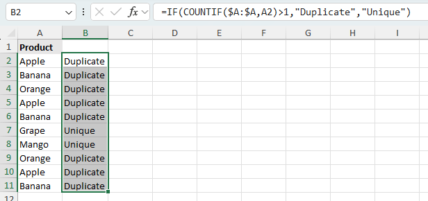
- Suppose the values you want to check are in column A, starting from cell A2.
- In the helper column beside the data, enter the following formula:
=IF(COUNTIF($A:$A,A2)>1,"Duplicate","Unique") - Press Enter, then drag the fill handle down to apply the formula to the other rows.
Excel will return Duplicate for values that appear more than once in the column, and Unique for values that appear only once.
Note:
If you do not want to display Unique for non-duplicate values, replace "Unique" with "" in the formula.
Pros
- Easy to set up
- Works well for single-column duplicate checks
- Updates automatically when the data changes
Label only the second and later duplicates
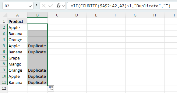
If you want to keep the first occurrence as the original and only mark the repeats, use this running COUNTIF formula.
- Assume the values are in column A, starting from A2.
- In the helper column, enter the formula below:
=IF(COUNTIF($A$2:A2,A2)>1,"Duplicate","") - Press Enter, then copy the formula downward.
With this method, the first occurrence remains blank, while the second and later occurrences are marked as Duplicate.
Note:
This is useful when you want to keep the first matching record as the main one and only flag the extra repeated entries.
Pros
- Keeps the first occurrence unmarked
- Useful for reviewing repeated records
- Easy to filter after labeling
Check for case-sensitive duplicates
Excel’s COUNTIF function is not case-sensitive, so values such as Apple and APPLE are treated as duplicates. If you need to distinguish values based on letter case, use a formula with EXACT.
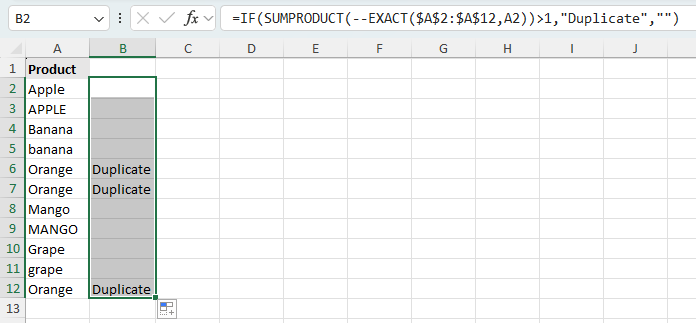
- Assume your values are in A2:A12.
- In the helper column, enter either of the formulas:
- Identify case-sensitive duplicates including 1st occurrences:
=IF(SUMPRODUCT(--EXACT($A$2:$A$12,A2))>1,"Duplicate","") - Identify case-sensitive duplicates excluding 1st occurrences:
=IF(SUMPRODUCT(--EXACT($A$2:A2,A2))>1,"Duplicate","")
- Identify case-sensitive duplicates including 1st occurrences:
- Press Enter, then fill the formula down.
These formulas check whether a value appears more than once with the exact same letter case. In the screenshot, I used the first formula, so all case-sensitive matches are marked as duplicates, including the first occurrence.
Note:
If you want to display Unique for non-duplicate values, replace "" with "Unique" in the formula.
Pros
- Can distinguish values by letter case
- Useful for codes, IDs, and text strings where case matters
Identify duplicates based on multiple columns
Sometimes a duplicate is not determined by one column alone. For example, a record may only be considered duplicated when both Product and Region match, or when an entire row is repeated. In that case, you need to check multiple columns together.
Use a formula to identify duplicate rows
This method uses COUNTIFS to test whether the combination of values in multiple columns appears more than once.
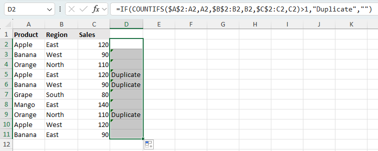
- Assume the duplicate check is based on columns A, B and C, starting from row 2.
- In a helper column, enter either of the following formulas:
- Identify duplicate rows including 1st occurrences:
=IF(COUNTIFS($A:$A,A2,$B:$B,B2,$C:$C,C2)>1,"Duplicate","") - Identify duplicate rows excluding 1st occurrences:
=IF(COUNTIFS($A$2:A2,A2,$B$2:B2,B2,$C$2:C2,C2)>1,"Duplicate","")
- Identify duplicate rows including 1st occurrences:
- Press Enter, then drag the formula down.
Excel will identify rows where the combination of values in columns A, B and C appears more than once. In the screenshot, I used the second formula, so the first occurrence of each matching row is left unmarked, while only the repeated rows are labeled as Duplicate.
$D:$D,D2, $E:$E,E2, and so on.Pros
- Works well for duplicate rows based on multiple fields
- Updates automatically when the data changes
- Flexible and easy to expand to more columns
Cons
- Requires a helper column
- Can become harder to read when many columns are involved
Identify duplicates across multiple columns with Kutools for Excel
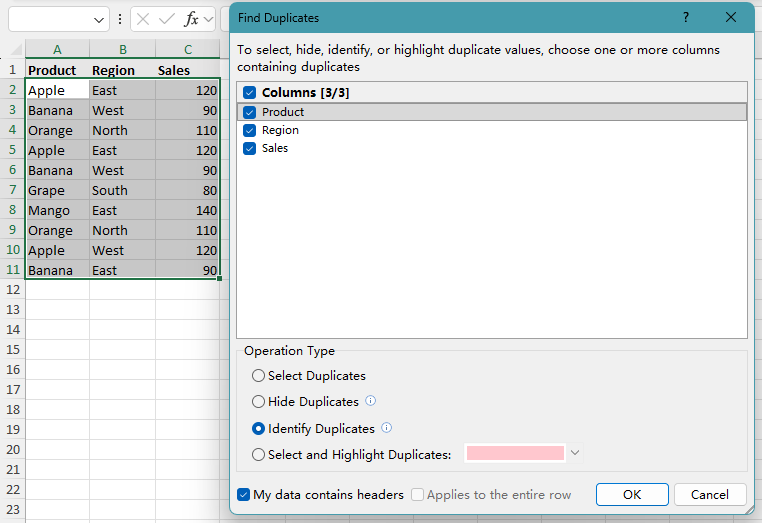
If you prefer not to use formulas, Kutools for Excel provides a built-in Find Duplicates feature that can identify duplicate rows based on one or more selected columns and add a label directly to the repeated records while leaving the first occurrence unmarked.
- Select the data range that you want to check for duplicates.
- Click Kutools > Find > Find Duplicates.
- In the Find Duplicates dialog box, check the columns that should be used to determine duplicate records.
- Under Operation Type, choose Identify Duplicates.
- Confirm whether your data contains headers, then click OK.

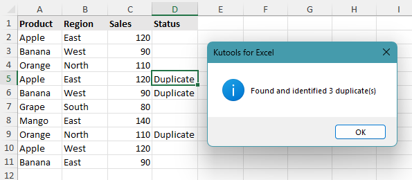
Kutools will identify duplicate rows based on the selected columns and insert the duplicate mark only beside the repeated records, excluding the first occurrence. As shown in the screenshot, Kutools also displays a confirmation dialog indicating how many duplicates were found.
Note:
This method is especially useful when you need to identify duplicates across many columns and want to avoid building long formulas manually.
Pros
- No formula writing required
- Can identify duplicates based on one or more columns
- Convenient for large or complex worksheets
Cons
- Requires Kutools for Excel
- Only supports excluding the first occurrence
Kutools for Excel - Packed with over 300 essential tools for Excel. Make Excel tasks faster, easier, and more efficient. Download now!
Frequently asked questions
What do the dollar signs in Excel formulas mean?
The dollar signs make a cell reference absolute. For example, $A$2 locks both the column and the row, so the reference does not change when you copy the formula down. This is useful when you want part of the formula range to stay fixed.
When should I include or exclude the first occurrence when identifying duplicates?
Include the first occurrence when you want to mark every matching value or record in the list. Exclude the first occurrence when you want to treat the first match as the original entry and mark only the repeated ones.
Why does Excel show a Formula Omits Adjacent Cells warning?
This warning can appear when a formula uses an expanding range on purpose, such as checking only the current row and the rows above it. In duplicate-checking formulas, this is often intentional, so the warning can usually be ignored.
Can I identify duplicates across multiple columns without formulas?
Yes. You can use Kutools for Excel to identify duplicate rows based on selected columns and add a duplicate mark directly to the worksheet without creating formulas manually.
Can Kutools for Excel identify duplicates in a list?
Yes. Kutools can identify duplicates in a single-column list by checking the column you choose, or across multiple columns by checking the selected fields together as one record.
Conclusion
Using formulas like COUNTIF and COUNTIFS gives you a flexible way to identify duplicates while keeping your data intact. For more advanced needs such as case-sensitive checks, combining functions like EXACT provides better control.
If you want a faster method without formulas, Kutools for Excel offers a simple way to label duplicates automatically.
I hope you found this tutorial helpful. If you’d like to explore more Excel tips and practical solutions, please click here to browse our full collection of Excel tutorials.
The Best Office Productivity Tools
Kutools for Excel - Helps You To Stand Out From Crowd
Kutools for Excel Boasts Over 300 Features, Ensuring That What You Need is Just A Click Away...
Office Tab - Enable Tabbed Reading and Editing in Microsoft Office (include Excel)
- One second to switch between dozens of open documents!
- Reduce hundreds of mouse clicks for you every day, say goodbye to mouse hand.
- Increases your productivity by 50% when viewing and editing multiple documents.
- Brings Efficient Tabs to Office (include Excel), Just Like Chrome, Edge and Firefox.
Table of Contents
- Identify duplicates (including 1st occurrences)
- Label only the second and later duplicates
- Check for case-sensitive duplicates
- Identify duplicates across multiple columns
- Use a formula to identify duplicate rows
- Identify duplicates across multiple columns with Kutools
- Frequently asked questions
- Conclusion
- The Best Office Productivity Tools
Kutools for Excel
Brings 300+ advanced features to Excel
- 🧩 Overview
- 📥 Free Download
- 🎁 30-Day Free Trial available