Find and Select Cells by Number Format in Excel (Currency, Percentage, etc.)
When working with reports in Excel, it is common to have different types of numbers in the same worksheet. Some cells show revenue or cost values in currency format, some show rates in percentage format, and others are regular numbers used for counts or quantities. In many cases, you may want to work with only one type of number format without manually checking each cell.
For example, you might want to copy only percentage-based metrics to another report, highlight all currency values for review, or quickly understand which parts of a sheet contain financial data and which parts contain performance data. Although Excel does not offer one direct command that instantly selects all currency or percentage cells together, there are several practical ways to do it.

In this tutorial, we will show you four practical ways to find and select cells with specific number formats in Excel, such as currency and percentage, using built-in tools, Kutools, the CELL function, and Conditional Formatting.
Find and select cells by picking a sample cell
This is the most practical built-in method in Excel. Instead of manually setting up the search format, you can simply click a cell that already uses the number format you want to find. Excel will then look for other cells with the same format, such as currency, percentage, date, or other number formats.
- Select the range to search, or skip this step to search the entire worksheet.
- Press Ctrl + F to open the Find and Replace dialog box.
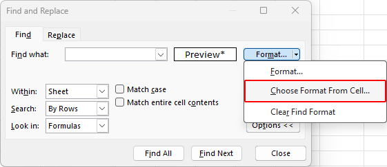
- Click Options >> to expand the dialog box.
- Click the arrow beside Format, then choose Choose Format From Cell.
- Click a cell that already uses the number format you want to find, such as a currency cell or a percentage cell.
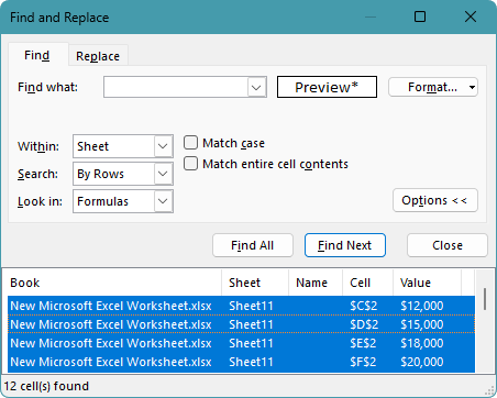
- Click Find All. Excel will list all matching cells at the bottom of the dialog box.
- Press Ctrl + A in the results list to select all found cells, then close the Find and Replace dialog box.


The cells with the selected number format will remain highlighted, and you can now apply an action such as changing the number format, adding a fill color, or copying them to another location.

Pros
- Built into Excel, so no add-in is required
- Fast and accurate for finding one specific number format
- Using a sample cell is easier than setting the format manually
Cons
- Can only search one format at a time
- Needs an existing sample cell if you use the faster shortcut
Quickly select cells with a specific number format using Kutools
If you want a faster and more visual way to find cells by number format, Kutools for Excel provides a convenient option. Its Highlight Number Formats feature can automatically identify the number formats used in a selected range, show them in a list, and highlight each format in a different color. You can then select all cells with a specific format, such as currency, percentage, date, or general, in one step.
- Click Kutools > Design View. Then select Highlight Number Formats on the Kutools Design tab.
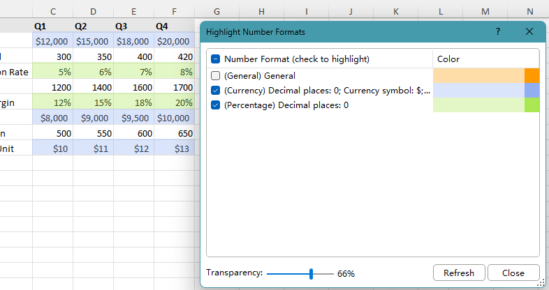
- When the Highlight Number Formats dialog box opens, it lists the number formats used in the worksheet and automatically highlights cells with different formats in different colors.
- Select the number format you want to work with, and all cells with that format will be selected at once.
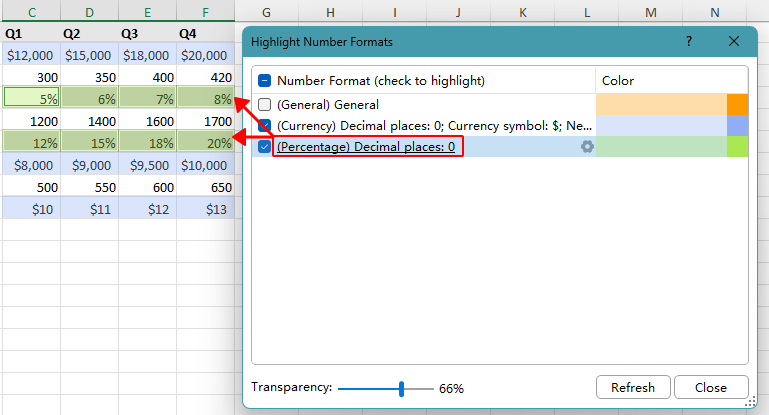
- You can now apply actions to the selected cells directly in the worksheet, such as formatting or copying them. Once done, you can select another number format in the dilaog box to continue if needed.


Note:
Kutools does not permanently change the cell style when highlighting number formats. The colors are only used for visual identification. If you uncheck a number format in the Highlight Number Formats dialog box or close the dialog, the highlight colors will disappear automatically.
Pros
- Faster and more user-friendly than repeated manual searches
- Helpful for large worksheets with mixed formatting
- Good choice for users who want a more visual workflow
Cons
- Requires installing Kutools for Excel
Kutools for Excel - Packed with over 300 essential tools for Excel. Make Excel tasks faster, easier, and more efficient. Download now!
Use the CELL function with Filter
If you want a more structured way to identify cells by number format, you can use the CELL function to return a format code for each cell, then filter the helper column to show only the formats you need. This method is especially useful when your dataset contains a mix of formats, such as Currency, Percentage, and General.
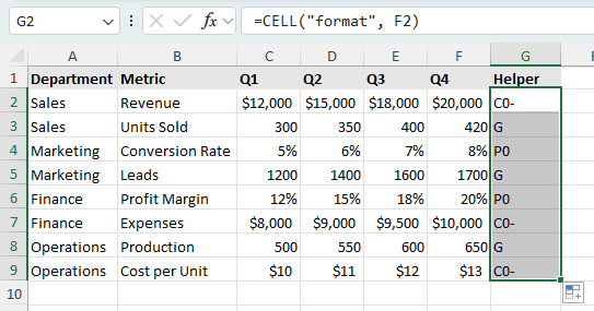
- Insert a blank helper column next to the data range you want to inspect.
- In the first helper cell, enter the following formula, replacing F2 with the first cell in the range you want to check for number formats:
=CELL("format", F2) - Press Enter, then drag the fill handle down to return the format code for the remaining cells in the range.
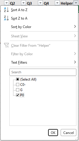
- Select the data range including the helper column, then click Data > Filter.
- Open the filter drop-down in the helper column, then select the format code you want to show. For example:
- C0- for Currency
- P0 for Percentage
- G for General
Tip: To understand the format codes returned by CELL("format", ...), refer to the CELL format code list.
- After filtering, the rows containing cells with the selected number format will be displayed, so you can review, copy, or work with them more easily.
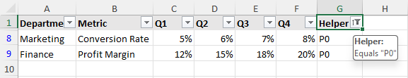


Note:
In addition to filtering, you can sort the helper column to group cells with the same number format together.
Pros
- Useful for analyzing formats across a dataset
- Works well when you want to review multiple format types
- Can be combined with sorting and filtering
Cons
- Less direct than the Find method
- Returned format codes are not always easy to interpret
- Requires an extra helper column
Use Conditional Formatting as a visual method
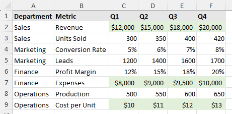
If you want to make cells with specific number formats stand out visually rather than select them right away, Conditional Formatting can be a useful alternative. This method works well when you want to scan a worksheet more easily and distinguish values such as currency, percentage, or other formats at a glance.
- Select the range you want to check.
- Click Home > Conditional Formatting > New Rule.
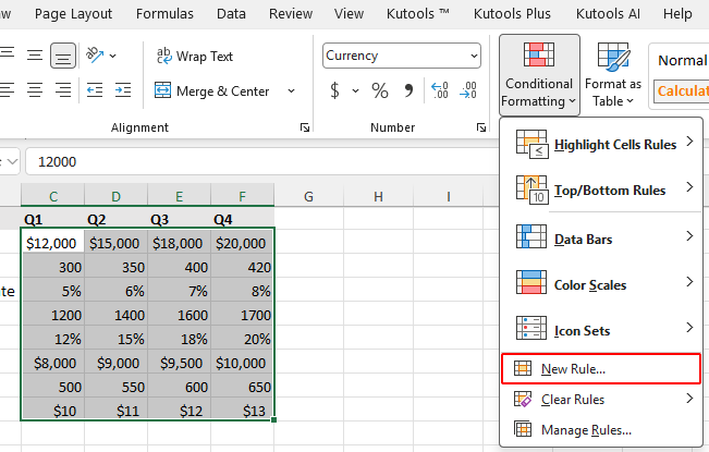
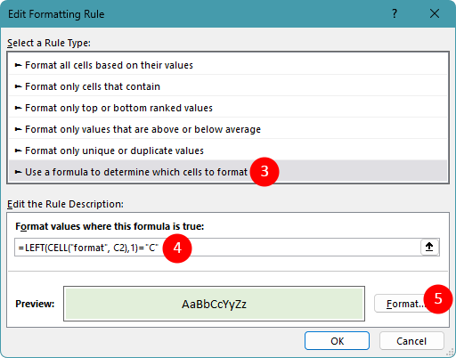
- Select Use a formula to determine which cells to format.
- Enter a formula to highlight the desired format:
- For percentage cells:
=LEFT(CELL("format", C2),1)="P" - For currency cells:
=LEFT(CELL("format", C2),1)="C"
Make sure to replace C2 with the first cell in your selected range.
- For percentage cells:
- Click Format and choose a fill color or font style, then click OK.
- Finally, click OK. After the target cells are highlighted, you can manually review them or work with them more easily.


This approach is best when you want a visual guide rather than a direct selection result.
Pros
- Good for visual review of large worksheets
- Makes currency or percentage cells easy to spot
- Helpful when you want to compare different types of values on screen
Cons
- Does not directly select cells by number format
- Requires basic formula knowledge to set up the highlighting rule
Which method works best for you?
| Method | Best for | Limitations |
|---|---|---|
| Find by picking a sample cell | Quickly finding one exact number format such as Currency or Percentage | Can only search one format at a time |
| Kutools for Excel | Users who want a faster or more visual selection workflow | Requires Kutools for Excel Download |
| CELL function + Filter | Analyzing and filtering number formats with a helper column | Less direct and needs extra setup |
| Conditional Formatting | Visually identify cells with specific number formats in a worksheet | Does not directly select cells by format |
Conclusion
If you want the simplest built-in way to find and select cells with a specific number format in Excel, using Find and picking a sample cell is usually the best choice. It is accurate, easy to use, and works well when you need to search for one format at a time.
For a faster and more visual experience, Kutools for Excel can make the process more convenient, especially when you often work with mixed number formats. The CELL function with Filter is a good option when you want to identify and organize formats more systematically, while Conditional Formatting is helpful when you simply want to make certain formats stand out visually.
I hope you found this tutorial helpful. If you’d like to explore more Excel tips and practical solutions, please click here to browse our full collection of Excel tutorials.
The Best Office Productivity Tools
Kutools for Excel - Helps You To Stand Out From Crowd
Kutools for Excel Boasts Over 300 Features, Ensuring That What You Need is Just A Click Away...
Office Tab - Enable Tabbed Reading and Editing in Microsoft Office (include Excel)
- One second to switch between dozens of open documents!
- Reduce hundreds of mouse clicks for you every day, say goodbye to mouse hand.
- Increases your productivity by 50% when viewing and editing multiple documents.
- Brings Efficient Tabs to Office (include Excel), Just Like Chrome, Edge and Firefox.
Table of Contents
- Select cells by picking a sample cell
- Quickly select cells using Kutools
- Identify and filter cells using the CELL function
- Use Conditional Formatting as a visual method
- Which method works best for you?
- Conclusion
- The Best Office Productivity Tools
Kutools for Excel
Brings 300+ advanced features to Excel
- 🧩 Overview
- 📥 Free Download
- 🎁 30-Day Free Trial available