How to Abbreviate Currency Values as K, M, and B in Excel?
Large currency values can make financial reports, dashboards, and sales worksheets difficult to scan. Instead of displaying amounts such as $125,000, $2,500,000, or $3,600,000,000, you can shorten them to:
| Original value | Abbreviated value |
|---|---|
| $125,000 | $125.0K |
| $2,500,000 | $2.5M |
| $3,600,000,000 | $3.6B |
The letters represent commonly used number units:
- K = thousand
- M = million
- B = billion
For example, $24.5K represents $24,500, while $3.2M represents $3,200,000.
In Excel, you can use a custom number format to change only how the values appear, a formula to generate abbreviated results in another column, or Kutools for Excel to format an entire range without memorizing format codes.
Abbreviate Currency Values with a Custom Number Format
Abbreviate Currency Values with a Custom Number Format
When all values in a range use the same unit, you can apply a simple custom number format to display them in thousands, millions, or billions.
This method changes only how the values appear. It does not divide, round, or replace the original numbers stored in the cells.
- Select the currency values you want to abbreviate.
- Press Ctrl + 1 to open the Format Cells dialog box.
- Select Custom from the Category list. And then enter the following code in the Type box:
✓ Format numbers in thousand:
$0.0,"K"✓ Format numbers in millions:
$0.0,,"M"✓ Format numbers in billions:
$0.0,,,"B"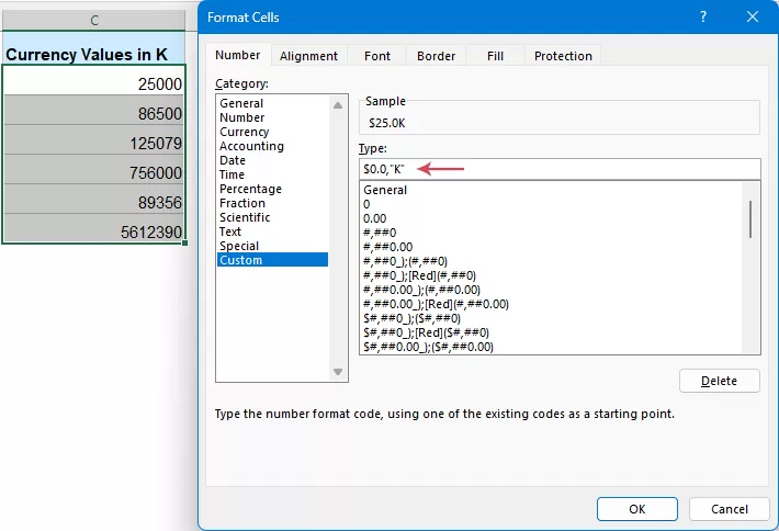
- Click OK.
Result: The values are now displayed in currency format and abbreviated as thousands, millions, or billions.
Display Currency Values in Thousands (K)--- $0.0,"K"
Display Currency Values in Millions (M)--- $0.0,,"M"
Display Currency Values in Billions (B)--- $0.0,,,"B"
Custom Currency Format Summary
| Display unit | Format code | Example |
|---|---|---|
| Thousands | $0.0,"K" | 125,000 → $125.0K |
| Millions | $0.0,,"M" | 8,500,000 → $8.5M |
| Billions | $0.0,,,"B" | 3,200,000,000 → $3.2B |
| Thousands without decimals | $0,"K" | 125,000 → $125K |
| Millions without decimals | $0,,"M" | 8,500,000 → $9M |
| Billions without decimals | $0,,,"B" | 3,200,000,000 → $3B |
| Millions with two decimals | $0.00,,"M" | 1,250,000 → $1.25M |
Changing the number of placeholders controls the displayed precision:
0displays no decimal places.0.0displays one decimal place.0.00displays two decimal places.0.#displays up to one decimal place without forcing a trailing zero.
For example:
$0.#,,"M"This displays 12,000,000 as $12M and 12,500,000 as $12.5M.
Use a Different Currency Symbol
When creating custom number formats in Excel, you are not limited to the dollar sign ($). You can easily use a different currency symbol depending on your region or reporting requirements.
To change the currency symbol, simply replace $ in the format code with the desired symbol. For example:
- Euros (€):
€0.0,"K" - British Pounds (£):
£0.0,,"M" - Japanese Yen (¥):
¥0,,,"B"
This allows the same K, M, and B abbreviation logic to work across different currencies while keeping your financial reports consistent and localized.
Automatically Display Currency Values as K, M, or B
A fixed number format works well when all values have a similar size. However, a dataset may contain thousands, millions, and billions in the same column. In this situation, you need a method that checks each value and applies the appropriate abbreviation automatically.
Method 1: Automatically Display K, M, or B with a Custom Number Format
A conditional custom number format can switch between thousands, millions, and billions according to the size of each value.
- Select the currency values you want to abbreviate.
- Press Ctrl + 1 to open the Format Cells dialog box.
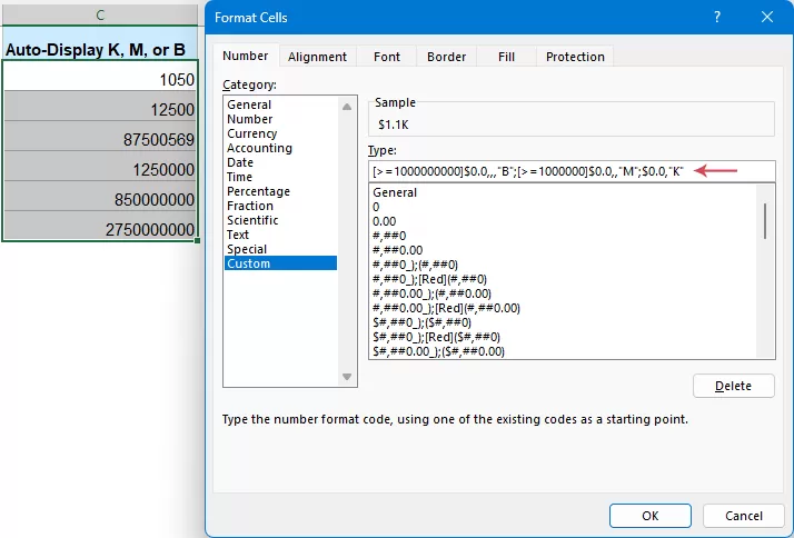
- Select Custom from the Category list. And then enter the following code in the Type box:
[>=1000000000]$0.0,,,"B";[>=1000000]$0.0,,"M";$0.0,"K"Tips: The format contains three sections:
[>=1000000000]$0.0,,,"B"Values of at least one billion are divided by one billion for display and followed by B.
[>=1000000]$0.0,,"M"Values of at least one million are divided by one million for display and followed by M.
$0.0,"K"All remaining values are divided by one thousand for display and followed by K.
- Click OK.
Result: The currency values are now automatically displayed as K, M, or B based on the values, while the original values remain unchanged.

Note: Prevent 999,999 from Appearing as 1000.0K
Because the format displays one decimal place, a value such as 999,999 may round to $1000.0K rather than switching to $1.0M.
To account for rounding near the unit boundaries, use adjusted thresholds:
[<999950]$0.0,"K";[<999950000]$0.0,,"M";$0.0,,,"B"This format produces more natural results when one decimal place is displayed:
| Original value | Result |
|---|---|
| 999,900 | $999.9K |
| 999,999 | $1.0M |
| 999,999,999 | $1.0B |
The adjusted threshold of 999,950 is used because values at or above that point round to 1,000.0K when displayed with one decimal place.
Advantages
- Keeps the original numeric values unchanged
- Works with calculations, PivotTables, and charts
- Requires no helper column
- Can be applied to an entire range at once
- Updates automatically when cell values change
Limitations
- Excel custom formats allow only two explicit conditions
- Values below 1,000 are displayed as fractions of K
- The format controls appearance only
- The displayed abbreviation cannot be extracted as text without another formula
Method 2: Automatically Add K, M, or B with a Formula
A formula is useful when you want the abbreviated result in a separate column or need more control over values below 1,000.
- Select a blank cell and copy and paste the following formula:
=IF(ABS(A2)>=1000000000,TEXT(A2/1000000000,"$0.0")&"B", IF(ABS(A2)>=1000000,TEXT(A2/1000000,"$0.0")&"M", IF(ABS(A2)>=1000,TEXT(A2/1000,"$0.0")&"K", TEXT(A2,"$0.00")))) - Press Enter, and then fill the formula down to apply the formula to the remaining rows.
- Select a blank cell and copy and paste the following formula:

How the Formula Works
The formula checks the absolute value of A2 from the largest unit to the smallest.
ABS(A2)>=1000000000
If the value is at least one billion, Excel divides it by one billion and adds B.
ABS(A2)>=1000000
If the value is at least one million, Excel divides it by one million and adds M.
ABS(A2)>=1000
If the value is at least one thousand, Excel divides it by one thousand and adds K.
TEXT(A2,"$0.00")
Values below 1,000 remain in the standard currency format.
The ABS function checks the size of both positive and negative values without removing the original negative sign.
Advantages
- Handles values below 1,000 separately
- Produces results in another column
- Allows customized symbols, units, and decimal places
- Can be adapted to more complex business rules
Limitations
- The result returned by TEXT is text rather than a numeric value
- The abbreviated results cannot be summed directly
- A helper column is required
- The formula is longer and more difficult to maintain
Method 3: Automatically Abbreviate Currency Values with Kutools for Excel
If you do not want to create custom format codes or maintain a nested formula, Kutools for Excel provides a quicker way to format large numbers.
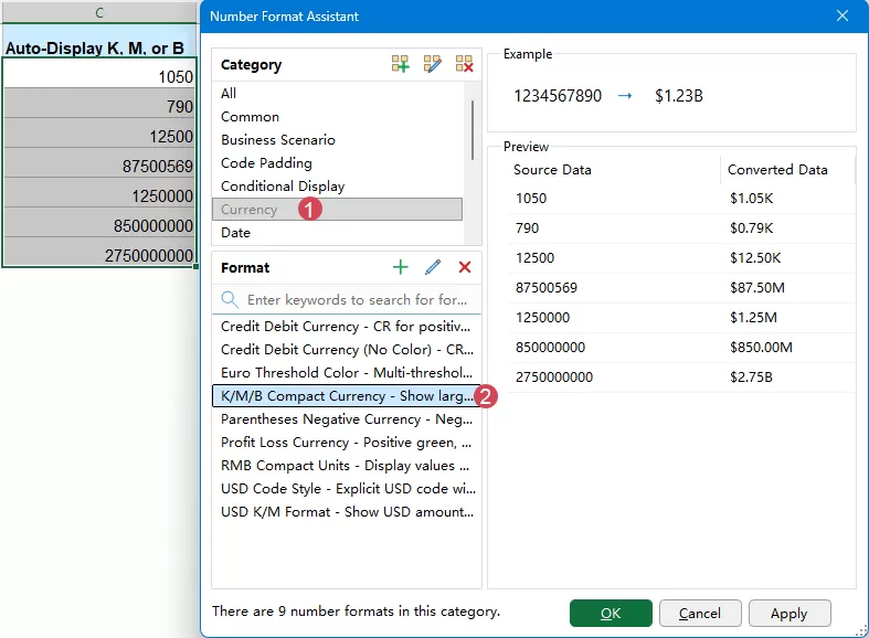
Kutools for Excel’s Number Format Helper provides ready-made currency formats, so you can shorten large values without entering custom format codes or formulas. With the K/B/M Compact Currency format, values below one million remain in standard currency format, while larger values are automatically displayed in millions or billions.
- Select the values you want to format.
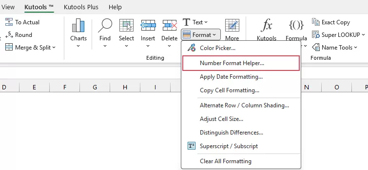
- Go to Kutools tab, and click Format > Number Format Helper, see screenshot:
- In the Number Number Format Assistant dialog box:
- In Category pane, select Currency.
- Choose K/M/B Compact Currency from the Format list. Check the converted results in the Preview pane.
- Click OK.
Result: The selected values are now displayed in a more compact currency format.

Kutools for Excel
Format large currency values quickly with ready-made formats—no complex formulas or custom format codes required.
- Format multiple currency values at once.
- Preview the results before applying the format.
- Keep the original numeric values unchanged and available for calculations.
- Choose from multiple ready-made currency formats.
Which Method Should You Use?
| Method | Keeps values numeric | Uses a helper column | Automatically switches units | Best for |
|---|---|---|---|---|
| Fixed custom format | Yes | No | No | Values using one consistent unit |
| Conditional custom format | Yes | No | Yes | Dashboards, reports, and charts |
| Formula | No, result is text | Yes | Yes | Customized output in another column |
| Kutools for Excel | Yes | No | Yes | Quick batch formatting without code |
Frequently Asked Questions
Conclusion
Abbreviating large currency values as K, M, and B can make Excel worksheets, dashboards, charts, and financial reports much easier to read.
- Use a fixed custom number format when all values should use the same unit.
- Use a conditional custom number format when Excel needs to switch automatically between thousands, millions, and billions while preserving the original numeric values.
- Use a formula when you need customized abbreviated results in a separate column or want values below 1,000 to remain unchanged.
- For a faster and more flexible solution without complex formulas or formatting codes, use Kutools for Excel.
By choosing the appropriate method, you can present large currency values clearly without changing the underlying financial data.
Best Office Productivity Tools
Supercharge Your Excel Skills with Kutools for Excel, and Experience Efficiency Like Never Before. Kutools for Excel Offers Over 300 Advanced Features to Boost Productivity and Save Time. Click Here to Get The Feature You Need The Most...
Office Tab Brings Tabbed interface to Office, and Make Your Work Much Easier
- Enable tabbed editing and reading in Word, Excel, PowerPoint, Publisher, Access, Visio and Project.
- Open and create multiple documents in new tabs of the same window, rather than in new windows.
- Increases your productivity by 50%, and reduces hundreds of mouse clicks for you every day!
All Kutools add-ins. One installer
Kutools for Office suite bundles add-ins for Excel, Word, Outlook & PowerPoint plus Office Tab Pro, which is ideal for teams working across Office apps.





- All-in-one suite — Excel, Word, Outlook & PowerPoint add-ins + Office Tab Pro
- One installer, one license — set up in minutes (MSI-ready)
- Works better together — streamlined productivity across Office apps
- 30-day full-featured trial — no registration, no credit card
- Best value — save vs buying individual add-in