How to Display Debit and Credit Values as DR and CR in Excel?
When working with accounting records, bank transactions, general ledgers, or trial balances, you may want Excel to display debit and credit amounts with the abbreviations DR and CR.
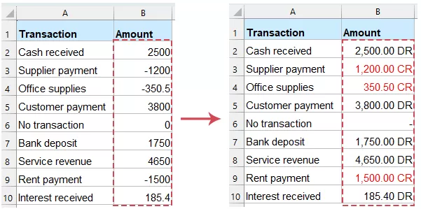
For example, the table below compares the original values with the results displayed after applying the DR and CR format:
| Transaction | Original Amount | Displayed Amount |
|---|---|---|
| Cash received | 2,500.00 | 2,500.00 DR |
| Supplier payment | -1,200.00 | 1,200.00 CR |
| No transaction | 0.00 | - |
Excel does not include a built-in DR/CR number format, but you can create one using a custom number format, a formula, or Kutools for Excel. This article explains each method in detail and helps you choose the most suitable solution.
What are Debit and Credit?
Debit and credit are the two sides of every accounting transaction.
A debit, commonly abbreviated as DR, records an amount on the debit side of an account. A credit, abbreviated as CR, records an amount on the credit side.
In many Excel worksheets, users adopt a simplified display convention:
- Positive values are displayed as debits with DR
- Negative values are displayed as credits with CR
- Zero values are displayed as a dash
This convention is useful for reports, but it should be applied according to the accounting structure used in your workbook.
Display Positive Values as DR and Negative Values as CR
Suppose the transaction amounts are stored in cells B2. Positive values represent debit amounts, while negative values represent credit amounts.
You can display them with DR and CR by using one of the following methods.
Method 1: Display DR and CR with a Custom Number Format
A custom number format is usually the best solution when you only want to change how the values appear without changing the underlying numbers.
Steps:
- Select the cells containing the numbers you want to format as debit and credit values.
- Press Ctrl + 1 to open the Format Cells dialog box.
- In the Category list, select Custom. And then, enter the following format code in the Type box:
#,##0.00 "DR";#,##0.00 "CR";"-"
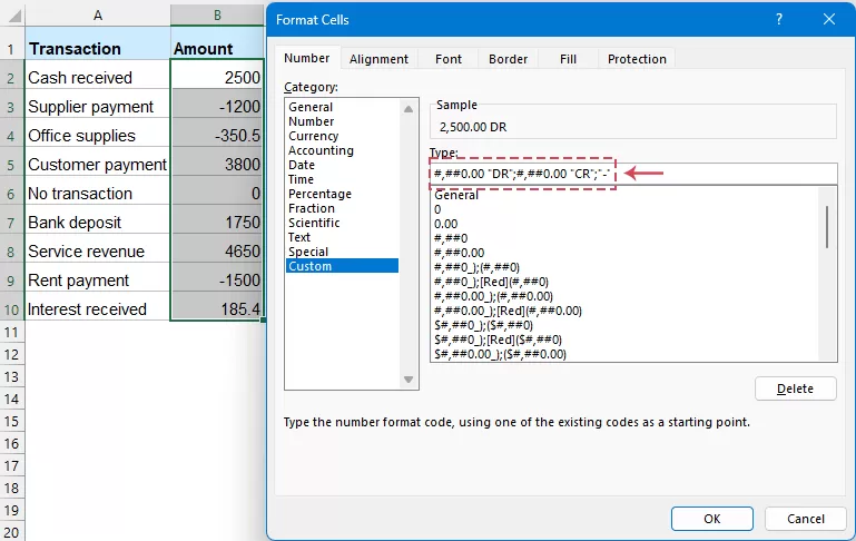
- Click OK. Excel will now display positive values as DR, negative values as CR, and zeros as a dash. See screenshot:
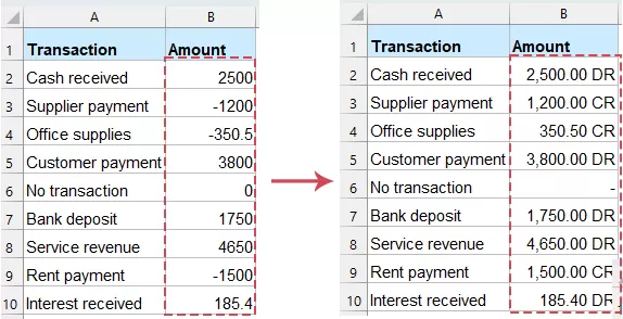
How the custom format works
- #,##0.00 "DR" formats positive values with two decimal places and adds DR.
- #,##0.00 "CR" formats negative values as positive-looking amounts and adds CR.
- "-" displays zero values as a dash.
Display values without decimal places
To display whole numbers only, use:
| Original Value | Displayed Value |
|---|---|
| 2500 | 2,500 DR |
| -1200 | 1,200 CR |
| 0 | - |
Display DR and CR in different colors
You can also add colors to the format:
Positive debit values will appear in blue, while negative credit values will appear in red.
| Original Value | Displayed Value |
|---|---|
| 2500 | 2,500 DR |
| -1200 | 1,200 CR |
| 0 | - |
Advantages
- Keeps the original numbers unchanged
- Works with SUM, AVERAGE, MAX, MIN, and other calculations
- Does not require a helper column
- Can be applied to an entire range at once
- Automatically updates when the values change
- Displays zero values as a clean dash
Limitation
- The format only changes the displayed result.
- DR and CR are not included when the cell is copied as plain text.
- Users may not realize that a displayed credit amount is still stored as a negative number.
Method 2: Display DR and CR with a Formula
Use a formula when you want the formatted debit and credit results to appear in a separate column. This method is useful when you need to export, print, concatenate, or combine the displayed values with other text.
Assume the original amount is in cell B2. Enter the following formula in D2:
=IF(B2=0,"-",TEXT(ABS(B2),"#,##0.00")&IF(B2>0," DR"," CR"))Press Enter, and then drag the fill handle down to apply the formula to the remaining rows. 
How the formula works?
- IF(B2=0,"-",...): If B2 contains zero, the formula returns a dash.
- ABS(B2): The ABS function removes the negative sign. Therefore, -1200 becomes 1200.
- IF(B2>0," DR"," CR"): If the value is greater than zero, the formula adds DR. If the value is less than zero, the formula adds CR.
- TEXT(ABS(B2),"#,##0.00"): The TEXT function formats the number with commas and two decimal places.
Formula without decimal places
To display whole numbers only, use the following formula:
Advantages
- Produces the formatted result in a separate column.
- DR and CR become part of the displayed text.
- Suitable for exporting values to text-based reports.
- Can be customized to show blanks, dashes, currency symbols, or additional descriptions.
- Does not change the original amount column.
Limitations
- Requires a helper column.
- The formula result is text rather than a numeric value.
- SUM and other mathematical functions cannot directly calculate the formatted results.
Method 3: Display DR and CR with Kutools for Excel
When you frequently apply specialized number formats, remembering and manually entering format codes can be inconvenient.
Kutools for Excel provides a more convenient way to manage and apply number formats through its Number Format Helper. It is especially useful when you regularly prepare accounting reports or need to process large ranges.
Steps:
- Select the cells containing the numbers you want to format as debit and credit values.
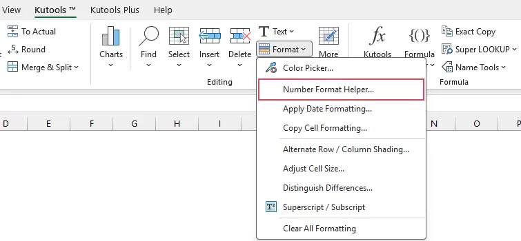
- Click Kutools > Format > Number Format Helper, see screenshot:
- In the Number Format Assistant dialog box, configure the following options:
- Select Currency from the Category box.
- Choose the required format from the Format list, such as :
Credit Debit Currency - CR for positive, DR for negative with red color
Credit Debit Currency (No Color) - CR for positive, DR for negative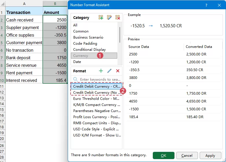
- Click OK to apply the format. The selected values will immediately display as DR or CR according to whether they are positive or negative. Zero values will display as a dash. See screenshot:
Why use Kutools for Excel?
Kutools is particularly useful when you need to work with many specialized number-formatting tasks.
- ✅️ A centralized interface for managing number formats
- ✅️ A preview of the formatting result before applying it
- ✅️ Faster processing of large data ranges
- ✅️ Less need to remember complex format codes
- ✅️ Easier access to other number-formatting tools
- ✅️ Suitable for users who frequently prepare reports and accounting worksheets
- ✅️ The underlying values remain numeric, so formulas and calculations continue to work normally.
Simplify number formatting and handle everyday Excel tasks more efficiently with Kutools for Excel.
Which method should you use?
| Method | Best For | Keeps Values Numeric | Helper Column Required | Main Advantage |
|---|---|---|---|---|
| Number format | Changing the appearance of existing values | Yes | No | Simple and built into Excel |
| Formula | Creating customized results in another column | No | Yes | Flexible output and text control |
| Kutools for Excel | Quickly applying and managing formats | Yes | No | Easier for frequent formatting tasks |
Frequently Asked Questions
1. Why does the negative amount appear without a minus sign?
The negative section of the custom number format does not contain a minus sign:
Excel therefore displays the absolute-looking amount followed by CR. However, the stored value remains negative.
For example, -1200 appears as 1,200.00 CR, but Excel still uses -1200 in calculations.
2. Does adding DR and CR change the original values?
It depends on the method. A custom number format or Kutools changes only the appearance of the value. The original number remains unchanged. A formula returns a text string such as 1,200.00 CR. The original value remains in the source cell, but the formula result is no longer numeric.
3. How can I display DR and CR before the amount?
- Use this custom number format:
"DR " #,##0.00;"CR " #,##0.00;"-"
4. Can I use parentheses for credit amounts?
Yes. Use:
A negative value such as -1200 will display as:
5. Does a positive value always mean debit?
No. Debit and credit treatment depends on the account type and the structure of the accounting system.
The methods in this article assume that your worksheet already uses positive numbers for debit entries and negative numbers for credit entries. If your data follows the opposite convention, reverse the DR and CR sections.
Conclusion
Displaying debit and credit amounts as DR and CR can make accounting worksheets clearer, more professional, and easier to review.
For most situations, use the following custom number format:
It displays positive values as DR, negative values as CR, and zero values as a dash while keeping the original numbers available for calculations.
Use a formula when you need customized text results in a separate column. For a faster and more convenient way to manage specialized number formats, use Kutools for Excel.
By choosing the appropriate method, you can create cleaner financial reports without changing the underlying accounting data.
Best Office Productivity Tools
Supercharge Your Excel Skills with Kutools for Excel, and Experience Efficiency Like Never Before. Kutools for Excel Offers Over 300 Advanced Features to Boost Productivity and Save Time. Click Here to Get The Feature You Need The Most...
Office Tab Brings Tabbed interface to Office, and Make Your Work Much Easier
- Enable tabbed editing and reading in Word, Excel, PowerPoint, Publisher, Access, Visio and Project.
- Open and create multiple documents in new tabs of the same window, rather than in new windows.
- Increases your productivity by 50%, and reduces hundreds of mouse clicks for you every day!
All Kutools add-ins. One installer
Kutools for Office suite bundles add-ins for Excel, Word, Outlook & PowerPoint plus Office Tab Pro, which is ideal for teams working across Office apps.





- All-in-one suite — Excel, Word, Outlook & PowerPoint add-ins + Office Tab Pro
- One installer, one license — set up in minutes (MSI-ready)
- Works better together — streamlined productivity across Office apps
- 30-day full-featured trial — no registration, no credit card
- Best value — save vs buying individual add-in