Merge Two Tables in Excel Based on One Key Column
Combining information from two tables is a common Excel task. For example, an order table may contain product IDs and quantities, while a separate product table stores the corresponding product names and prices. The VLOOKUP to merge two tables based on one key column function in Kutools for Excel's Formula Helper Plus retrieves matching information from one table and adds it to another. You only need to specify the return range, lookup value, lookup range, and match type. Kutools for Excel then creates the INDEX and MATCH formula automatically.
- What VLOOKUP to merge two tables based on one key column can do
- Benefits of VLOOKUP to merge two tables based on one key column
- How to use VLOOKUP to merge two tables based on one key column in the Formula Helper Plus
- Tips for better results
- Best use cases
- About Formula Helper Plus
- Frequently Asked Questions
Benefits of VLOOKUP to merge two tables based on one key column
Formula Helper Plus makes it easier to bring related fields into a second table while keeping the result connected to the source data.
No formula memorization
Select the required cells and ranges without remembering how to write or combine the INDEX and MATCH functions.
Fill multiple records efficiently
Create the formula for the first record and copy it down. The lookup value changes for each row while the source ranges remain fixed.
Enter a value or use a cell reference
Enter the lookup value directly or select a worksheet cell so the lookup value and returned result can change dynamically.
Support threshold-based matching
Use match type 1 or -1 to merge records with sorted reference tables based on minimum thresholds or maximum limits.
Return values from either side
The generated INDEX and MATCH formula can return values from a range located to the left or right of the lookup range.
Keep results connected to source data
The returned results update automatically when the referenced lookup values or source values change.
How to use VLOOKUP to merge two tables based on one key column in the Formula Helper Plus
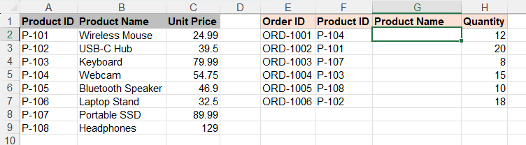
In this example, the product table in A2:C9 contains product IDs, names, and unit prices. The order table contains product IDs and quantities but does not include product names. We will match the Product ID in each order and return the corresponding Product Name.
- Select the first empty cell in the column where you want to return the matching values. In this example, select G2.
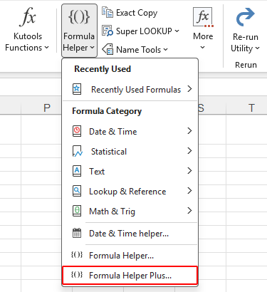
- Click Kutools > Formula Helper > Formula Helper Plus.
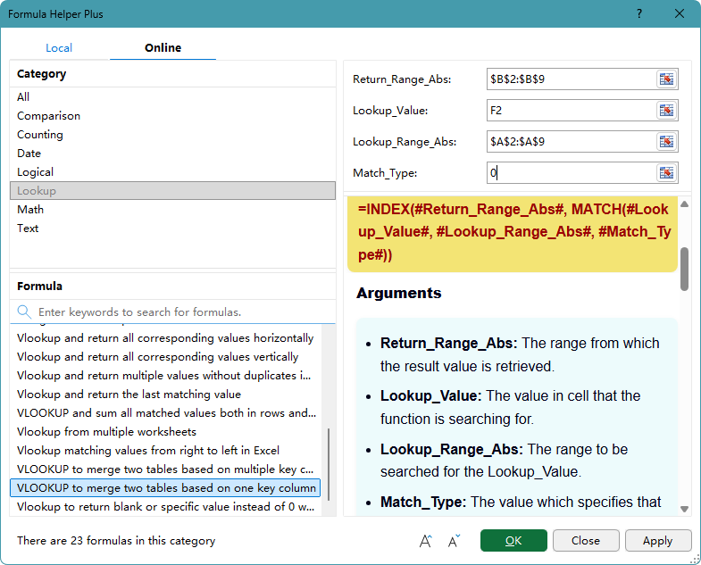
- In the Formula Helper Plus dialog box, on the Online tab, select the Lookup category, and then select VLOOKUP to merge two tables based on one key column.
- Configure the arguments as follows:
- Return_Range_Abs: Select B2:B9, which contains the product names to return.
- Lookup_Value: Select F2, which contains the Product ID to find.
- Lookup_Range_Abs: Select A2:A9, which contains the Product IDs in the product table.
- Match_Type: Enter 0 to require an exact match.
- Click OK. Kutools inserts the formula in G2, returns Webcam, and closes the dialog box.
- Copy the formula down to the remaining cells in the Product Name column. Excel returns the product name that matches each Product ID.
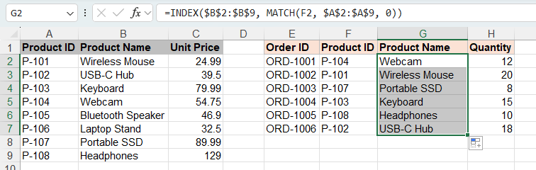
Kutools creates the following formula for the first order:
=INDEX($B$2:$B$9,MATCH(F2,$A$2:$A$9,0))The MATCH function finds the position of the Product ID in F2 within A2:A9. The INDEX function then returns the product name from the same position in B2:B9. For Product ID P-104, the formula returns Webcam.
📝 Notes:
- When the formula is copied down, the lookup value changes from F2 to F3, F4, and so on. The return and lookup ranges use absolute references, so they remain unchanged.
- In this example, the lookup value is stored in a worksheet cell so each copied formula can use the Product ID from its own row.
- Instead of selecting a cell that contains the lookup value, you can enter a value directly in the Lookup_Value box. However, a directly entered value remains the same when the formula is copied.
Tips for better results
Use consistent keys and correctly aligned ranges to obtain reliable matches.
- Use a shared key: Both tables must contain a column with matching values, such as Product ID. The column headings do not have to be identical, but the values used for matching must correspond.
- Keep the ranges the same size: Return_Range_Abs and Lookup_Range_Abs must contain the same number of rows so each lookup value aligns with the correct return value.
- Use 0 for exact matching: By default, use 0 to merge records by an exact matching key. You can also use 1 or -1 when the key column represents sorted thresholds or ranges rather than unique identifiers.
- Check the data type: A number stored as text will not always match the same number stored as a numeric value. Make sure the key columns use consistent data types.
- Remove unintended spaces: Leading or trailing spaces in text-based keys can cause an exact lookup to return #N/A.
- Use unique keys when possible: If the lookup range contains duplicates, the formula returns the value associated with the first match.
Best use cases
This function is primarily designed to merge two tables by an exact shared key. It can also merge records by sorted thresholds when the reference table uses ranges instead of unique identifiers.
Add product details to orders
Merge an order table with a product table by matching Product IDs, and return information such as product names, categories, or unit prices.
Add employee details to reports
Merge a report with an employee table by matching Employee IDs, and return departments, job titles, office locations, or other employee information.
Add customer tiers by spending
Merge a customer table with a tier table that stores ascending minimum spending requirements and the corresponding membership levels.
Add shipping rates by weight
Merge an order table with a shipping table that stores descending maximum weight limits and the rate assigned to each weight band.
About Formula Helper Plus
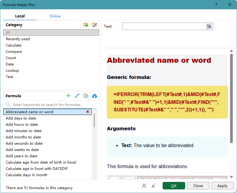
Formula Helper Plus is a formula library in Kutools for Excel that helps you find and insert useful formulas through a guided interface. Formulas are organized into categories, and each one provides labeled argument boxes and instructions explaining the required inputs. You can also create categories and formulas for calculations you use regularly, or share useful formulas to help expand the Online formula library.
- 🗂️ Category tools
- Category list: Browse formulas by category, such as Calculate, Compare, Count, Date, Lookup, and Text.
- Add category
 : Create a category for organizing your own formulas.
 - Rename category
 : Select a custom category, and click this button to rename it.
- 🧮 Formula tools
- Search: Enter keywords in the search box to find a formula by its name or purpose.
- Add formula
 : Create a formula and assign it to a category. When defining the formula, enclose each variable argument in # signs, such as #Range#.
 - Edit formula
 : Select a custom formula, and click this button to modify its formula, category, or description.
 - Copy formula
 : Create an editable copy of the selected formula. This is useful when you want to build a new formula based on an existing one.
 - Upload formula
 : Upload and share the selected formula to help us expand the Online formula library.
 : Create a category for organizing your own formulas.
 : Select a custom category, and click this button to rename it.
 : Create a formula and assign it to a category. When defining the formula, enclose each variable argument in # signs, such as #Range#.
 : Select a custom formula, and click this button to modify its formula, category, or description.
 : Create an editable copy of the selected formula. This is useful when you want to build a new formula based on an existing one.
 : Upload and share the selected formula to help us expand the Online formula library.
Frequently Asked Questions
Why does the formula return #N/A?
The lookup value may not exist in the selected lookup range, or the values may have inconsistent data types or extra spaces. Confirm that the key exists and that both tables store it in the same format.
Why does the formula return the wrong value?
Check that Return_Range_Abs and Lookup_Range_Abs start and end on corresponding rows. If the ranges are misaligned, INDEX may return a value from the wrong record.
What happens when the lookup range contains duplicate keys?
The formula returns the value associated with the first matching key. Use unique IDs when every record must return one specific result.
Can the return range be to the left of the lookup range?
Yes. The generated INDEX and MATCH formula can return values from a range located either to the left or right of the lookup range.
Will copied formulas use the correct lookup value for each row?
Yes, if Lookup_Value refers to a worksheet cell. The relative cell reference changes as the formula is copied, while the absolute source ranges remain fixed.
Does the formula update when the source table changes?
Yes. If a value in the referenced return range changes, Excel recalculates the formula and displays the updated result.
The Best Office Productivity Tools
Kutools for Excel - Helps You To Stand Out From Crowd
Kutools for Excel Boasts Over 300 Features, Ensuring That What You Need is Just A Click Away...
Office Tab - Enable Tabbed Reading and Editing in Microsoft Office (include Excel)
- One second to switch between dozens of open documents!
- Reduce hundreds of mouse clicks for you every day, say goodbye to mouse hand.
- Increases your productivity by 50% when viewing and editing multiple documents.
- Brings Efficient Tabs to Office (include Excel), Just Like Chrome, Edge and Firefox.
Table of Contents
- What VLOOKUP to merge two tables based on one key column can do
- Benefits of VLOOKUP to merge two tables based on one key column
- How to use VLOOKUP to merge two tables based on one key column in the Formula Helper Plus
- Tips for better results
- Best use cases
- About Formula Helper Plus
- Frequently Asked Questions
Kutools for Excel
Brings 300+ advanced features to Excel
- 🧩 Overview
- 📥 Free Download
- 🎁 30-Day Free Trial available