How to create timeline (milestone) chart template in Excel?

The first section will guide you to prepare data for a timeline/milestone chart creating in Excel.

Step 1: Prepare a table and enter your original data as the following screen shot shown:

Step 2: Add height values for each event in the Column E. You’d better mix the negative numbers and positive numbers in the column.

Step 3: Specify the Axis values for each event. In Cell F2 enter =A2+(DATE(1900,IF(B2="",1,B2),0)+C2)/365.25, and drag the Fill Handle down to apply this formula to the range you want.

Step 4: Specify the Label values for each event. In Cell G2 enter =OFFSET(D2,ROW()-ROW(G2),0,1,1), and drag the Fill handle down to apply this formula to the range you want.

Then you will get a table similar as the following screen shot shown:

---

Part 2: Create a timeline/milestone chart in Excel

With the first part we have prepared a table (see screen shot above) for timeline/milestone chart creating. And this part will walk you through creating a timeline/milestone chart in Excel.

Step 1: Don’t select any content in the table, and click the Insert > Scatter (or Insert Scatter(X, Y) or Bubble Chart button in Excel 2013)> Scatter. See screen shot below:

Step2: Right click the blank chart, and select the Select Data from the right-clicking menu.

Step 3: In the opening Select Data Source dialog box, click the Add button. Then in the Edit Series dialog box,

(1) In the Series name box enter a name for this series, such as Timeline;

(2) Specify the Range F2:F14 in Axis column as the X values in the Series X values box;

(3) Specify the Range E2:E14 in Height column as the Y values in the Series Y values box;

(4) Click both OK buttons to close two dialog boxes.

Step 4: Add error bars for the scatter chart:

1. In Excel 2013, select the scatter chart, and click the Design > Add Chart Element > Error Bars > More Error Bars Options;
2. In Excel 2007 and 2010, select the scatter chat, and click the Layout > Error Bars > More Error Bars Options.

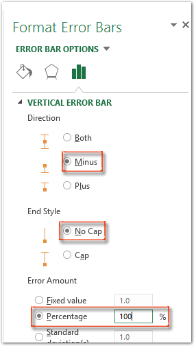
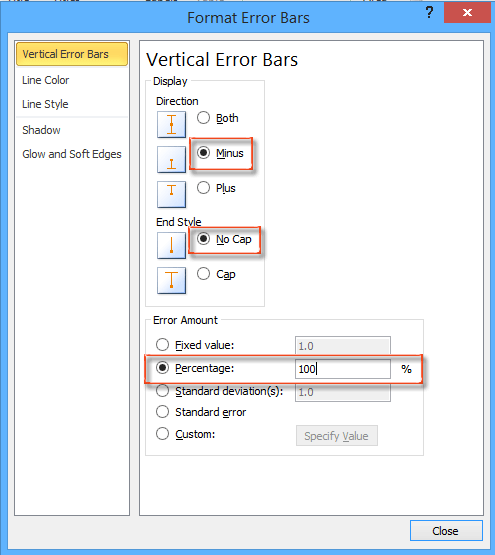
Step 5: In the coming Format Error Bars dialog box/pane, click the Vertical error bar tab, and check the Minus option, No Cap option, and Percentage option, and specify 100% in the percentage box. Then close the dialog box or pane.

Excel 2013 and higher versions:

Excel 2007 and 2010:

Step 6: Go to the scatter chart, click any horizontal line at the top of error bars, and press the Delete key.

Step 7: Right click any data point, and select the Add Data Labels from the right-clicking menu.

Next click one data label twice, and in the formula bar enter =, select the corresponding label in the Label column, and press the Enter key. And repeat this step to change each data point’s label one by one.

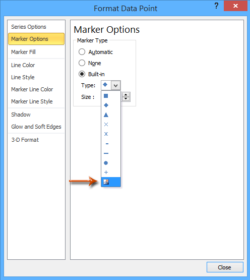
Step 8: Click one data point twice, right click and select the Format Data Point from the right-clicking menu.

Step 9: Add a picture or photo for selected data point:

1. In Excel 2013’s Format Data Point pane, click the Fill & Line tab > Marker > Marker Options > Built-in, then click the Type box and specify the image icon from the drop down list;
2. In Excel 2010/2007’s Format Data Point dialog box, click the Marker Options tab > Built-in, then click the Type box and specify the image icon from the drop down list.

Excel 2013 and higher versions:

Excel 2007 and 2010:

Step 10: In the opening Insert Picture dialog box, find out the image or photo you will add for selected data point, and click the Insert button.

 Notes:

(1) We can’t adjust the image size after inserting into chart, as a result, we have to prepare the images in proper size before the step 9.

(2) We can also insert an image by this way: select the scatter chart, click Insert > Picture and find out a corresponding image, and then resize and move this image in the chart.

Step 11: Repeat the Step 8 – Step 10 to add images for each data point one by one, and then close the Format Data Point dialog box/pane.

This part will show you how to save the timeline chart as a chart template in Excel easily.

Step 1: Save the timeline/milestone chart as a chart template:

1. In Excel 2013, right click the timeline chart, and select the Save as Template from the right-clicking menu.
2. In Excel 2007 and 2010, click the timeline chart to activate the Chart Tools, and then click the Design > Save As Template.

Step 2: In the popping up Save Chart Template dialog box, enter a name for your template in the File name box, and click the Save button.

How to make a read-only template in Excel?

How to protect/lock an Excel template being overwritten with password?

How to find and change default save location of Excel templates?

How to edit/change a personal template in Excel?

How to change the default workbook/sheet template in Excel?