Three Types of Multi-Column Drop Down Lists – Step by Step Guide
When you search for “excel drop down list multiple columns” on Google, you may need to achieve one of the following tasks:
In this tutorial, we will demonstrate step-by-step how to achieve these three tasks.
Make a Dependent Drop-Down List Based on Multiple Columns
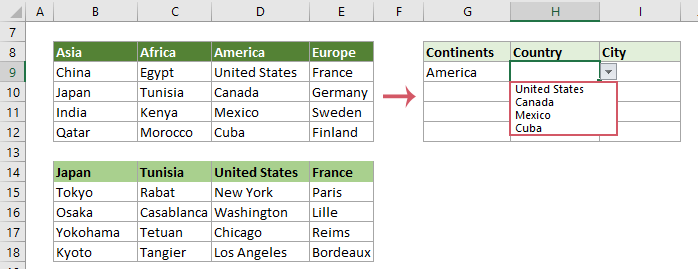
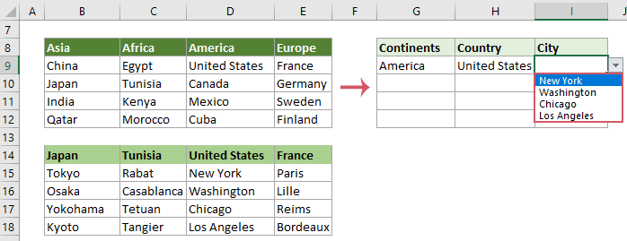
As shown in the GIF image below, you want to create a main drop-down list for the continents, a secondary drop-down list containing countries based on the continent selected in the main drop-down list, and then the third drop-down list containing cities based on the country selected in the secondary drop-down list. The method in this section can help you achieve this task.
Using formulas to make a dependent drop-down list based on multiple columns
Step 1: Create the main drop-down list
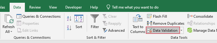
1. Select the cells (here I select G9:G13) where you want to insert the drop-down list, go to the Data tab, click Data Validation > Data Validation.
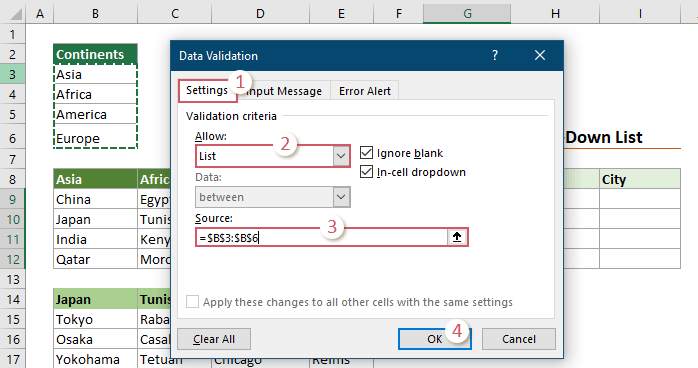
2. In the Data Validation dialog box, please configure as follows.
Step 2: Create the secondary drop-down list
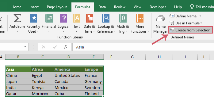
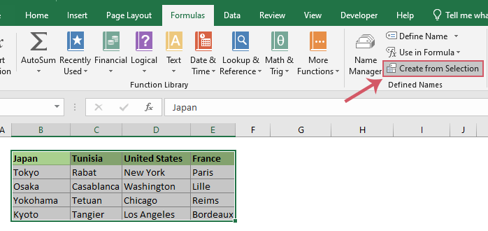
1. Select the entire range that contains the items you want to display in the secondary drop-down list. Go to the Formulas tab, and then click Create from Selection.
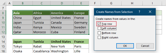
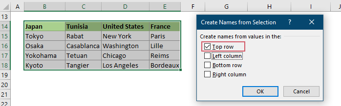
2. In the Create Names from Selection dialog box, only check the Top row box and then click the OK button.
3. Select a cell where you want to insert the secondary drop-down list, go to the Data tab, click Data Validation > Data Validation.
4. In the Data Validation dialog box, you need to:
=INDIRECT(SUBSTITUTE(G9," ","_"))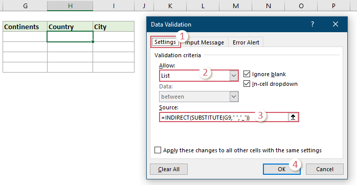
5. Select this drop-down list cell, drag its AutoFill Handle down to apply it to other cells in the same column.
The secondary drop-down list is now complete. When you select a continent in the main drop-down list, only the countries under this continent are displayed in the secondary drop-down list.
Step 3: Create the third drop-down list
1. Select the entire range that contains the values you want to display in the third drop-down list. Go to the Formulas tab, and then click Create from Selection.
2. In the Create Names from Selection dialog box, only check the Top row box and then click the OK button.
3. Select a cell where you want to insert the third drop-down list, go to the Data tab, click Data Validation > Data Validation.
4. In the Data Validation dialog box, you need to:
=INDIRECT(SUBSTITUTE(H9," ","_"))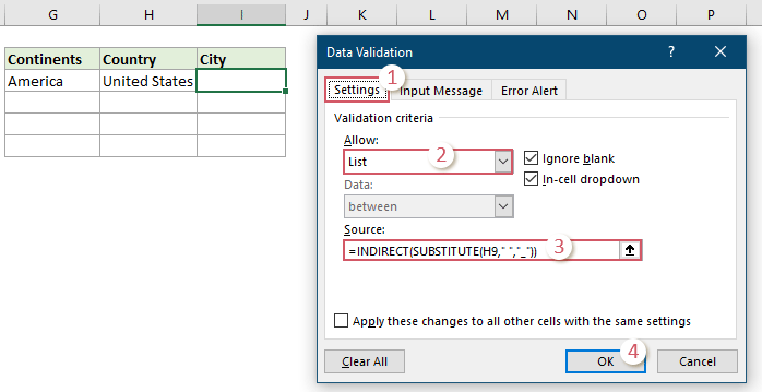
5. Select this drop-down list cell, drag its AutoFill Handle down to apply it to other cells in the same column.
The third drop-down list containing cities is now complete. When you select a country in the secondary drop-down list, only the cities under this country are displayed in the third drop-down list.
The above method might be cumbersome for some users, if you want a more efficient and straightforward solution, the following method can be achieved with just a few clicks.
A few clicks to create a dependent drop-down list based on multiple columns with Kutools for Excel
The GIF image below shows the steps of the Dynamic Drop Down List feature of Kutools for Excel.
As you can see, the whole operation can be done in just a few clicks. You just need to:
The GIF image above only demonstrates the steps to make a 2-level drop-down list. If you want to make a drop-down list with more than 2 levels, click here to know more. Or download the 30-day free trial.
Make Multiple Selections in a Drop-Down List in Excel
This section provides two methods to help you make multiple selections in a drop-down list in Excel.
Using VBA codes to make multiple selections in an Excel drop-down list
The following VBA script can help to make multiple selections in a drop-down list in Excel without duplicates. Please do as follows.
Step 1: Open the VBA code editor and copy the code
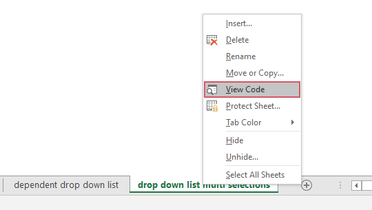
1. Go to the sheet tab, right click on it and select View Code from the right-clicking menu.
2. Then the Microsoft Visual Basic for Applications window pops up, you need to copy the following VBA code in the Sheet (Code) editor.
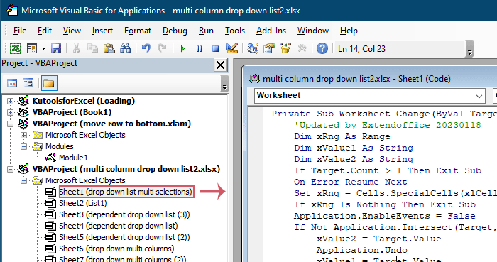
VBA code: Allow multiple selections in a drop-down list without duplicates
Private Sub Worksheet_Change(ByVal Target As Range)
    'Updated by Extendoffice 2019/11/13
    Dim xRng As Range
    Dim xValue1 As String
    Dim xValue2 As String
    If Target.Count > 1 Then Exit Sub
    On Error Resume Next
    Set xRng = Cells.SpecialCells(xlCellTypeAllValidation)
    If xRng Is Nothing Then Exit Sub
    Application.EnableEvents = False
    If Not Application.Intersect(Target, xRng) Is Nothing Then
        xValue2 = Target.Value
        Application.Undo
        xValue1 = Target.Value
        Target.Value = xValue2
        If xValue1 <> "" Then
            If xValue2 <> "" Then
                If xValue1 = xValue2 Or _
                   InStr(1, xValue1, ", " & xValue2) Or _
                   InStr(1, xValue1, xValue2 & ",") Then
                    Target.Value = xValue1
                Else
                    Target.Value = xValue1 & ", " & xValue2
                End If
            End If
        End If
    End If
    Application.EnableEvents = True
End Sub
Step 2: Test the code
After pasting the code, press the Alt + Q keys to close the Visual Editor and go back to the worksheet.
Tips: This code works for all drop-down lists in the current worksheet. Just click a cell containing the drop-down list, select items one by one from the drop-down to test if it works.
A few clicks to make multiple selections in an Excel Drop-down list with Kutools for Excel
VBA code has many limitations. If you are not familiar with VBA script, it is hard to modify the code to meet your needs. Here is a recommended powerful feature - Multi-selection Drop-down List that can help you easily select multiple items from drop-down list.
After installing Kutools for Excel, go to the Kutools tab, select Drop-down list > Multi-select Drop-down List. Then configure as follows.
- Specify the range containing the drop-down list from which you need to select multiple items.
- Specify the separator for the selected items in the drop-down list cell.
- Click OK to complete the settings.


Result
Now, when you click on a cell with a drop-down list in the specified range, a list box will appear next to it. Simply click the "+" button next to the items to add them to the drop-down cell, and click the "-" button to remove any items you don't want anymore. See the demo below:
- Check the Wrap Text After Inserting a Separator option if you want to display the selected items vertically within the cell. If you prefer a horizontal listing, leave this option unchecked.
- Check the Enable search option if you want to add a search bar to your drop-down list.
- To apply this feature, please download and install Kutools for Excel first.
Display Multiple Columns in a Drop-Down List
As shown in the screenshot below, this section is going to show you how to display multiple columns in a drop-down list.
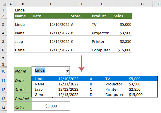
By default, a data validation drop-down list displays only one column of items. To display multiple columns in a drop-down list, we recommend using a Combo Box (ActiveX Control) instead of a data validation drop-down list.
Step 1: Insert a Combo Box (ActiveX Control)
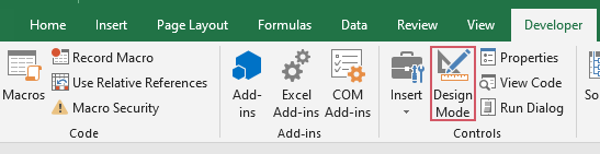
1. Go to the Developer tab, click Insert > Combo Box (ActiveX Control).
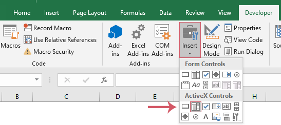
Tips: If the Developer tab does not display in the ribbon, you can follow the steps in this tutorial “Show Developer tab” to show it.
2. Then draw a Combo Box in a cell where you want to display the drop-down.
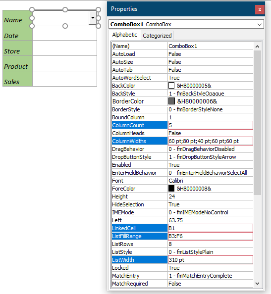
Step 2: Change the Properties of the Combo Box
1. Right click the Combo Box then select Properties from the context menu.
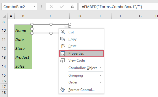
2. In the Properties dialog box, please configure as follows.
Step 3: Display the specified columns in the drop-down list
1. Under the Developer tab, turn off the Design Mode by just clicking the Design Mode icon.
2. Click the arrow of the combo box, the list will be expanded and you can see the specified number of columns being displayed in the drop-down.
Step 4: Show items from other columns in certain cells
1. Select a cell under the combo box, enter the formula below and press the Enter key to get the value of the second column in the same row.
=IFERROR(VLOOKUP(B1,B3:F6,2,FALSE),"")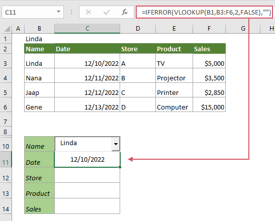
2. To get the values of the third, fourth and fifth columns, apply the following formulas one by one.
=IFERROR(VLOOKUP(B1,B3:F6,3,FALSE),"")=IFERROR(VLOOKUP(B1,B3:F6,4,FALSE),"")=IFERROR(VLOOKUP(B1,B3:F6,5,FALSE),"")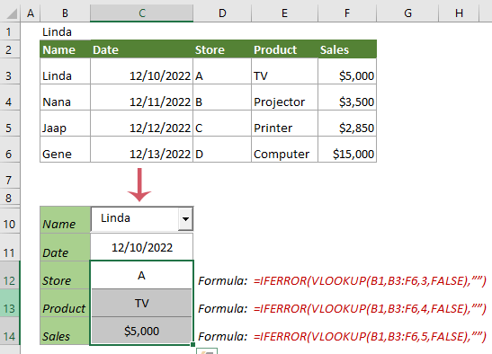
Related Articles
Autocomplete when typing in Excel drop down list
If you have a data validation drop down list with large values, you need to scroll down in the list just for finding the proper one, or type the whole word into the list box directly. If there is method for allowing to auto complete when typing the first letter in the drop down list, everything will become easier. This tutorial provides the method to solve the problem.
Create drop down list from another workbook in Excel
It is quite easy to create a data validation drop down list among worksheets within a workbook. But if the list data you need for the data validation locates in another workbook, what would you do? In this tutorial, you will learn how to create a drop fown list from another workbook in Excel in details.
Create a searchable drop down list in Excel
For a drop down list with numerous values, finding a proper one is not an easy work. Previously we have introduced a method of auto completing drop down list when enter the first letter into the drop down box. Besides the autocomplete function, you can also make the drop down list searchable for enhancing the working efficiency in finding proper values in the drop down list. For making drop down list searchable, try the method in this tutorial.
Auto populate other cells when selecting values in Excel drop down list
Let’s say you have created a drop down list based on the values in cell range B8:B14. When you selecting any value in the drop down list, you want the corresponding values in cell range C8:C14 be automatically populated in a selected cell. For solving the problem, the methods in this tutorial will do you a favor.
Best Office Productivity Tools
Supercharge Your Excel Skills with Kutools for Excel, and Experience Efficiency Like Never Before. Kutools for Excel Offers Over 300 Advanced Features to Boost Productivity and Save Time. Click Here to Get The Feature You Need The Most...
Office Tab Brings Tabbed interface to Office, and Make Your Work Much Easier
- Enable tabbed editing and reading in Word, Excel, PowerPoint, Publisher, Access, Visio and Project.
- Open and create multiple documents in new tabs of the same window, rather than in new windows.
- Increases your productivity by 50%, and reduces hundreds of mouse clicks for you every day!
All Kutools add-ins. One installer
Kutools for Office suite bundles add-ins for Excel, Word, Outlook & PowerPoint plus Office Tab Pro, which is ideal for teams working across Office apps.
- All-in-one suite — Excel, Word, Outlook & PowerPoint add-ins + Office Tab Pro
- One installer, one license — set up in minutes (MSI-ready)
- Works better together — streamlined productivity across Office apps
- 30-day full-featured trial — no registration, no credit card
- Best value — save vs buying individual add-in