Excel drop down list: create, edit, remove and more advanced operations

A drop-down list is similar to list box that allows users to pick one value from a selection list. This tutorial is going to demonstrate the basic operations for drop-down list: create, edit and remove drop down list in excel. Apart from that, this tutorial provides advanced operations for drop-down list to enhance its functionality to solve more Excel issues.

Create simple drop down list

For using a drop down list, you need to learn how to create it firstly. This section provides 6 ways to help you create a drop-down list in Excel.

Create drop down list from a range of cells

Here, we'll demonstrate the steps to create a drop-down list from a cell range in Excel. Please do as follows

1. Select a cell range to place the drop down list.

Tips: You can create a drop-down list for multiple non-contiguous cells at the same time by holding the "Ctrl" key while selecting the cells one by one.

2. Click "Data" > "Data Validation" > "Data Validation".

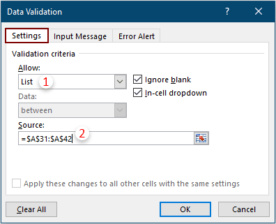
3. In the "Data Validation" dialog box, under the "Settings" tab, please configure as follows.

Notes:

Now the drop down list is created. When clicking the drop down list cell, an arrow will display next to it, click the arrow to expand the list, and then you can choose an item from it.

Create dynamic drop down list from table

You can convert your data range to an Excel table and then create a dynamic drop down list based on the table range.

1. Select the original data range, and then press the "Ctrl" + "T" keys.

2. Click "OK" in the popping up "Create Table" dialog box. Then the data range is converted to table.

3. Select a cell range for putting the drop-down list, and then click "Data" > "Data Validation" > "Data Validation".

4. In the "Data Validation" dialog box, you need to:

Then, dynamic drop-down lists are created. When adding or removing data from the table range, values in drop-down list will be updated automatically.

Create dynamic drop down list with formulas

Apart from creating dynamic drop down list from table range, you can also use a formula to create a dynamic drop down list in Excel.

1. Select the cells where to output the drop down lists.

2. Click "Data" > "Data Validation" > "Data Validation".

3. In the "Data Validation" dialog box, please configure as follows.

=OFFSET($A$13,0,0,COUNTA($A$13:$A$24),1)

Then, dynamic drop-down lists are created. When adding or removing data from the specific range, values in drop-down lists will be updated automatically.

Create drop down list from named range

You can also create a drop-down list from a named range in Excel.

1. Firstly, create a named range. Select the cell range you will create named range based on, and then type in the range name into the "Name" box, and press "Enter" key.

2. Click "Data" > "Data Validation" > "Data Validation".

3. In the "Data Validation" dialog box, please configure as follows.

Now the drop down list using data from a named range is created.

Create drop down list from another workbook

Supposing there is a workbook named “SourceData”, and you want to create a drop-down list in another workbook based on data in this "SourceData” workbook, please do as follows.

1. Open the “SourceData” workbook. In this workbook, select the data you will create a drop-down list based on, type a range name into the "Name" box, and then press the "Enter" key.

Here I name the range as City.

2. Open the worksheet you will insert drop down list. Click "Formulas" > "Define Name".

3. In the "New Name" dialog box, you need to create a named range based on the range name you created in workbook “SourceData”, please configure as follows.

=SourceData.xlsx!City

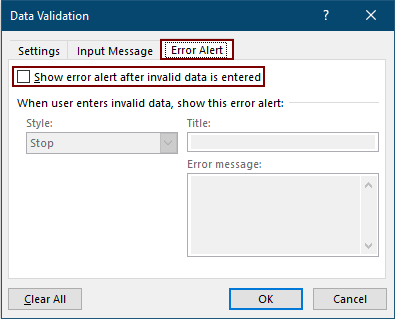
Notes:

4. Open the workbook you will insert drop down list, select the cells for the drop down list, and then click "Data" > "Data Validation" > "Data Validation".

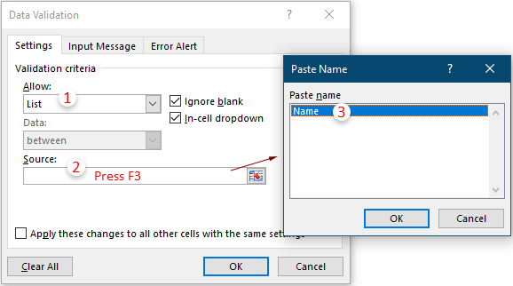
5. In the "Data Validation" dialog box, please configure as follows.

Now the drop down lists have been inserted in selected range. And the drop-down values are from another workbook.

Easily create a drop-down list with an amazing tool

Here, I highly recommend the "Create simple drop-down list" utility of "Kutools for Excel". With this feature, you can easily create drop-down list with specific cell values or create drop-down list with custom lists preset in Excel.

1. Select the cells you want to insert drop-down list, and then click "Kutools" > "Drop-down List" > "Create simple drop-down list".

2. In the "Create simple drop down list" dialog box, please configure as follows.

Note: If you want to create a drop-down list based on a custom list preset in Excel, please select the "Custom Lists" option in the "Source" section, choose a custom list in the "Custom Lists" box, and then click the "OK" button.

Now the drop down lists have been inserted in selected range.

Edit drop down list

If you want to edit drop down list, methods in this section can do you a favor.

Edit a drop down list based on a cell range

For editing a drop down list based on a cell range, please do as follows.

1. Select the cells containing drop down list you want to edit, and then click "Data" > "Data Validation" > "Data Validation".

2. In the "Data Validation" dialog box, change the cell references in the "Source" box and then click the "OK" button.

Edit a drop down list based on a named range

Supposing you add or delete values in the named range, and the drop down list is created based on this named range. For appearing the updated values in drop down lists, please do as follows.

1. Click "Formulas" > "Name Manager".

Tips: You can open the "Name Manager" window by pressing the "Ctrl" + "F3" keys.

2. In the "Name Manager" window, you need to configure as follows:

2.1) In the "Name" box, select the named range you want to update;

2.2) In the "Refers to" section, click the button to select the updated range for your drop down list;

2.3) Click the "Close" button.

3. Then a "Microsoft Excel" dialog box pops up, click the "Yes" button to save the changes.

Then drop down lists based on this named range are updated.

Remove drop down list

This section is talking about removing drop down list in Excel.

Remove drop down list with Excel built-in feature

Excel provides a built-in feature to help removing drop down list from worksheet. Please do as follows.

1. Select the cell range containing the drop down list you want to remove.

2. Click "Data" > "Data Validation" > "Data Validation".

3. In the "Data Validation" dialog box, click the "Clear All" button, and then click "OK" to save the changes.

Now drop down lists are removed from the selected range.

Easily remove drop down lists with an amazing tool

"Kutools for Excel" provides a handy tool - "Clear Data Validation Restrictions" to help easily remove drop down list from one or multiple selected ranges at once. Please do as follows.

1. Select the cell range containing the drop down list you want to remove.

2. Click "Kutools" > "Prevent Typing" > "Clear Data Validation Restrictions". See screenshot:

3. Then a "Kutools for Excel" dialog box pops up to ask you if clear the drop down list, please click the "OK" button.

Then drop down lists in this selected range are removed immediately.

Add color to drop down list

In some cases, you may need to make a drop down list that is color-coded in order to distinguish the data in the drop down list cells at a glance. This section provides two methods to help you solve the problem in detail.

Add color to drop down list with Conditional Formatting

You can create conditional rules to the cell containing the drop down list to make it color-coded. Please do as follows.

1. Select the cells containing the drop down list that you want to make it color-coded.

2. Click "Home" > "Conditional Formatting" > "Manage Rules".

3. In the "Conditional Formatting Rues Manager" dialog box, click the "New Rule" button.

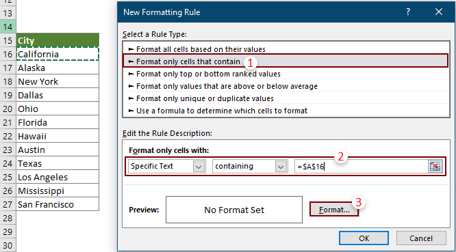
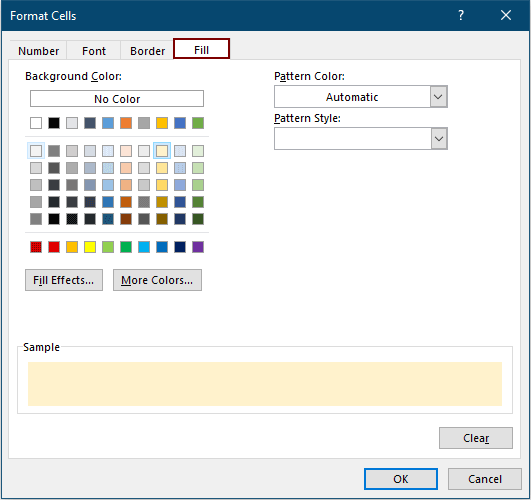
4. In the "New Formatting Rule" dialog box, please configure as follows.

4.1) In the "Select a Rule Type" box, choose the "Format only cells that contain" option;

4.2) In the" Format only cells with" section, select "Specific Text" from the first drop down list, select "containing" from the second drop down list, and then select the first item of the source list in the third box;

Tips: Here I select cell A16 in the third text box. A16 is the first item of the source list that I created drop down list based on.

4.3) Click the "Format" button.

4.4) In the "Format Cells" dialog box, go to the "Fill" tab, choose a background color for the specified text, and then click the "OK" button. Or you can choose a certain font color for the text as you need.

4.5) Click the "OK" button when it returns to the "New Formatting Rule" dialog box.

5. When it returns to the "Conditional Formatting Rules Manager" dialog box, repeat the above steps 3 and 4 to specify colors for other drop down items. After finish specifying colors, click the "OK" to save the changes.

From now on, when selecting an item from the drop down list, the cell will be highlighted with specified background color based on the selected text.

Easily add color to drop down list with an amazing tool

Here we introduce the "Colored Drop-down List" feature of "Kutools for Excel" to help you easily add color to drop down list in Excel.

1. Select the cells containing the drop down list that you want to add color.

2. Click "Kutools" > "Drop-down List "> "Colored Drop-down List".

3. In the "Colored Drop-down list" dialog box, please do as follows.

Tips: If you want to highlight rows based on drop down list selection, please choose the "Row of data range" option in the "Apply to" section, and then select the rows you will highlight in the "Highlight rows" box.

Now the drop down lists are color-coded as the below screenshots shown.

Highlight cells based on drop-down list selection

Highlight rows based on drop-down list selection

Create dependent drop down list in Excel or Google Sheets

A dependent drop down list helps to display choices depending on the value seletced in the first drop down list. If you need to create a dependent (cascarding) drop down list in Excel worksheet or in Google Sheets, methods in this section can do you a favor.

Create a dependent drop down list in Excel worksheet

The below demo displays the dependent drop down list in Excel worksheet.

Please click How To Create Dependent Cascading Drop Down List In Excel? for a step-by-step guide tutorial.

Create a dependent drop down list in Google Sheets

If you want to create a dependent drop down list in Google Sheets, please see How To Create A Dependent Drop Down List In Google Sheet?

Create searchable drop down lists

For the drop down lists containing long list of items in a worksheet, it’s not easy for you to pick up a certain item from the list. If you remember the initial characters or several consecutive characters of an item, you can do the search feature in a drop down list to easily filter it. This section is going to demonstrate how to create a searchable drop down list in Excel.

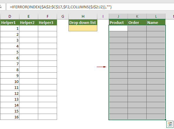
Supposing the source data you want to create a drop-down list based on is located in column A of Sheet1 as the below screenshot shown. Please do as follows to create a searchable drop down list in Excel with these data.

1. Firstly, create a helper column beside the source data list with an array formula.

In this case, I select cell B2, enter the below formula into it and then press the "Ctrl" + "Shift" + "Enter" keys to get the first result.

=IFERROR(INDEX($A$2:$A$50,SMALL(IFERROR(MATCH(IF(FIND(CELL("contents"),$A$2:$A$50)>0,$A$2:$A$50,""),$A$2:$A$50,0),""),ROW(A1))),"")

Select the first result cell, and then drag its "Fill Handle" all the way down until it reaches the end of the list.

Note: In this array formula, $A$2:$A$50 is the source data range on which you will create a drop-down list. Please change it based on your data range.

2. Click "Formulas" > "Define Name".

3. In the "Edit Name" dialog box, please configure as follows.

=OFFSET(Sheet1!$B$2,0,0,COUNTA(Sheet1!$B$2:$B$50)-COUNTIF(Sheet1!$B$2:$B$50,""),1)

Now you need to create the drop down list based on the named range. In this case, I will create searchable drop down list in Sheet2.

4. Open the Sheet2, select the range of cells for the drop down list, and then click "Data" > "Data Validation" > "Data Validation".

5. In the "Data Validation" dialog box, please do as follows.

5.1) In the "Allow" box, select "List";

5.2) Click the "Source" box, and then press the "F3" key;

5.3) In the popping up "Paste Name" dialog, select the named range you created in step3 and then click "OK";

Tips: You can directly enter the named range as "=named range" into the "Source" box.

5.4) Click the "Error Alert" tab, uncheck the" Show error alert after invalid data is entered" box, and finally click the "OK" button.

6. Right click the sheet tab (Sheet2) and select "View Code" from the right-clicking menu.

7. In the opening "Microsoft Visual Basic for Applications" window, copy the below VBA code into the Code editor.

VBA code: create searchable drop down list in Excel

Private Sub Worksheet_SelectionChange(ByVal Target As Range)
Application.Calculate
End Sub

8. Press the "Alt" + "Q" keys to close the "Microsoft Visual Basic for Appliations" window.

Now the searchable drop down lists are created. If you want to pick up an item, just enter one or several consecutive characters of this item into the drop down cell, click the drop down arrow, and then the item based on the entered content are listed in the drop down list. See screenshot:

Note: This method is case-sensitive.

Create drop down list but show different values

Supposing you have created a drop down list, when selecting an item from it, you want something else display in the cell. As the below demo shown, you have created drop down list based on the country name list, when selecting country name from the drop down, you want to display the abbreviation of the selected country name in the drop down cell. This section provides VBA method to help you solve the problem.

1. On the right side of the source data (the country name column), create a new column containing the abbreviation of the country names that you want to display in the drop down cell.

2. Select both the country name list and the abbreviation list, type a name in the "Name" box and then press the "Enter" key.

3. Select the cells for the drop down list (here I select D2:D8), and then click "Data" > "Data Validation" > "Data Validation".

4. In the "Data Validation" dialog box, please configure as follows.

5. After creating the drop down list, then right click the sheet tab and then select "View Code" from the right-clicking menu.

6. In the opening "Microsoft Visual Basic for Applications" window, copy the below VBA code into the Code editor.

VBA code: Show different values in drop down list

Private Sub Worksheet_Change(ByVal Target As Range)
'Updateby Extendoffice 20201027
    selectedNa = Target.Value
    If Target.Column = 4 Then
        selectedNum = Application.VLookup(selectedNa, ActiveSheet.Range("dropdown"), 2, False)
        If Not IsError(selectedNum) Then
            Target.Value = selectedNum
        End If
    End If
End Sub

Notes:

7. Press the "Alt" + "Q" keys to close the "Microsoft Visual Basic for Applications" window.

From now on, when selecting a certain country name from the drop down list, the corresponding abbreviation of the selected country name will be displayed in the cell.

Create a drop down list with checkboxes

Many Excel users tend to create a drop-down list with multiple checkboxes so that they can select multiple items from the list by just ticking the checkboxes.

As the below demo shown, when clicking the cell containing drop down list, a listbox appears. In the listbox, there is a checkbox before each item. You can tick the checkboxes to display the corresponding items in the cell.

If you want to create a drop down list with checkboxes in Excel, please see How To create a drop-down list With Multiple Checkboxes In Excel?.

Add autocomplete to drop down list

If you have a data validation drop down list with large items, you need to scroll up and down in the list for finding the proper one, or type the whole word into the list box directly. If the drop-down list can autocomplete when typing the first letter in it, everything will become easier.

For making drop down list autocomplete in a worksheet in Excel, please see How To Autocomplete When Typing In Excel Drop Down List?.

Filter data based on drop down list selection

This section will demonstrate how to apply formulas to create a drop down list filter in order to extract data based on the selection from the drop down list.

1. Firstly you need to create a drop down list with the specific values you will extract data based on.

Tips: Please follow the above steps to create a drop down list in Excel.

Create a drop down list with a unique list of items

If there are duplicates in your range, and you don’t want to create a drop down list with repetition of an item, you can create a unique list of items as follows.

1) Copy the cells you will create a drop-down list based on with "Ctrl" + "C" keys, and then paste them to a new range.

2) Select the cells in the new range, click "Data" > "Remove Duplicates".

3) In the "Remove Duplicates" dialog box, click the "OK" button.

4) Then a "Microsoft Excel" pops up to tell you how many duplicates are removed, click "OK".

Now you get the unique list of items, you can create a drop-down list based on this unique list now.

2. Then you need to create three helper columns as follows.

2.1) For the first helper column (here I choose column D as the first helper column), enter the below formula into the first cell (except the column header), and then press the "Enter" key. Select the result cell and then drag the "Fill Handle" all the way down until it reaches the bottom of the range.

=ROWS($A$2:A2)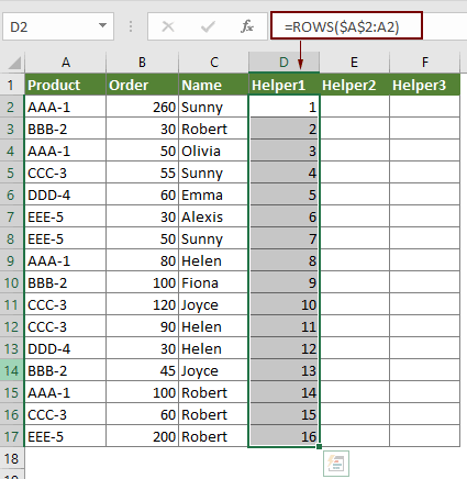

2.2) For the second helper column (the E column), enter the below formula in cell E2 and then press the "Enter" key. Select E2 and then drag the "Fill Handle" to the bottom of the range.

Note: If no value selected in the drop down list, here the results of formulas will display as blank.

=IF(A2=$H$2,D2,"")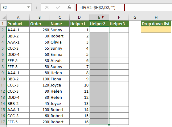

2.3) For the third helper column (the F column), enter the below formula in F2 and then press the "Enter" key. Select F2 and then drag the "Fill Handle" to the bottom of the range.

Note: If no value selected in the drop down list, the results of formulas will display as blank.

=IFERROR(SMALL($E$2:$E$17,D2),"")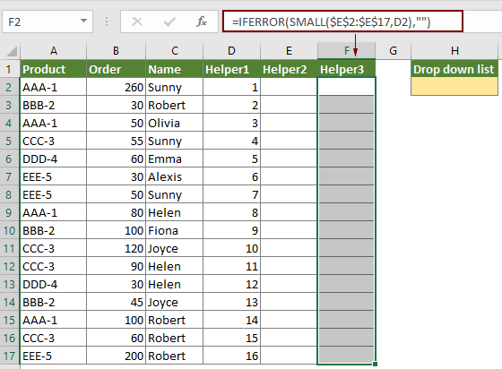

3. Create a range based on the original data range to output the extracted data with the below formulas.

3.1) Select the first output cell (Here I select J2), enter the below formula into it and then press the "Enter" key.

=IFERROR(INDEX($A$2:$C$17,$F2,COLUMNS($J$2:J2)),"")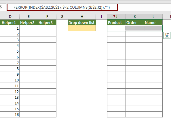

3.2) Select the result cell, and then drag the" Fill Handle" across to the right two cells.

3.3) Keep the range J2:l2 selected, drag the Fill Handle all the way down until it reaches the bottom of the range.

Notes:

Now a drop down list filter is created, you can easily extract data from the original data range based on the drop down list selection.

Select multiple items from drop down list

By default, the drop down list allows users to select only one item per time in a cell. When reselecting item in a drop down list, the previously selected item will be overwritten. However, if you are asked to select multiple items from a drop down list and display all of them in the drop down cell as the below demo shown, how can you do?

For selecting multiple items from drop down list in Excel, please see How To create a drop-down list With Multiple Selections Or Values In Excel?. This tutorial provides two methods in detail to help you solve the problem.

Set default (preselected) value for drop down list

By default, a drop down list cell displays as blank, the drop down arrow only appears when you click on the cell. How to figure out which cells contain drop down lists in a worksheet at a glance?

This section will demonstrate how to set default (preselected) value for drop down list in Excel. Please do as follows.

Before applying the below two methods, you need to create a drop-down list and do some configurations as follows.

1. Select the cells for the drop down list, click "Data" > "Data Validation" > "Data Validation".

Tips: If you have already created drop down list, please select the cells containing the drop down list, and then click "Data" > "Data Validation" > "Data Validation".

2. In the "Data Validation" dialog box, please configure as follows.

2.1) In the "Allow" box, select "List";

2.2) In the "Source" box, select the source data you will display in the drop down list.

Tips: For the drop down list you have already created, please skip these two steps.

2.3) Then go to the "Error Alert" tab, uncheck the "Show error alert after invalid data is entered" box;

2.4) Click the "OK" button.

After creating the drop down list, please apply one of the below methods to set default value for them.

Set default value for drop down list with formula

You can apply the below formula to set default value for the drop down list you created as the above steps shown.

1. Select the drop down list cell, enter the below formula into it and then press the "Enter" key to display the default value. If the drop down list cells are consecutive, you can drag the "Fill Handle" of the result cell to apply the formula to other cells.

=IF(C2="", "--Choose item from the list--")

Notes:

Set default value for all drop down lists in a worksheet at once with VBA code

Supposing there are lots of drop-down lists located in different ranges in your worksheet, to set the default value for all of them, you need to apply the formula repeatedly. That’s time-consuming. This section provides a useful VBA code for you to set default value for all drop down lists in a worksheet at once.

1. Open the worksheet containing the drop down lists you want to set default value, press the "Alt" + "F11" keys to open the "Microsoft Visual Basic for Applications" window.

2. In the "Microsoft Visual Basic for Applications" window, click "Insert" > "Module", and then paste the below VBA code into the Code window.

VBA code: Set default value for all drop down lists in a worksheet at once

Sub SetDropDownListToDefaultValue()
'Updated by Extendoffice 20201026
Dim xWs As Worksheet
Dim xRg, xFRg As Range
Dim xET: xET = Null
Dim xStr As String
xStr = "- Choose from the list -"
Set xWs = Application.ActiveSheet
Set xRg = xWs.UsedRange.Cells
    On Error Resume Next
    For Each xFRg In xRg
    xET = Null
    xET = xFRg.Validation.Type
    If Not IsNull(xET) Then
        If xFRg.Validation.Type = 3 Then
            xFRg.Value = "'" & xStr
        End If
    End If
    Next
End Sub

Notes: In the above code, "- Choose from the list -" is the default value to display in the drop down list cell. You can also change the default value based on your need.

3. Press the "F5" key, then a Macros dialog box pops up, make sure the "DropDownListToDefault" is selected in the "Macro Name" box, and then click the "Run" button to run the code.

Then the specified default value is populated into drop down list cells immediately.

Increase drop down list font size

Normally, drop down list has a fixed font size, if the font size is too small to read, you can try the below VBA method to enlarge it.

1. Open the worksheet containing the drop down lists you want to enlarge the font size, right click the sheet tab and then select" View Code" from the right-clicking menu.

2. In the "Microsoft Visual Basic for Applications" window, copy the below VBA code into the Code editor.

VBA code: Enlarge the font size of drop down lists in a worksheet

Private Sub Worksheet_SelectionChange(ByVal Target As Range)
'updateby Extendoffice 20201027
    On Error GoTo LZoom
    Dim xZoom As Long
    xZoom = 100
    If Target.Validation.Type = xlValidateList Then xZoom = 130
LZoom:
    ActiveWindow.Zoom = xZoom
End Sub

Note: Here, "xZoom = 130" in the code means that you will enlarge the font size of all drop-down lists in the current worksheet to 130. You can change it as you need.

3. Press the "Alt" + "Q" keys to close the "Microsoft Visual Basic for Applications" window.

From now on, when clicking on the drop down cell, the zoom level of current worksheet will be enlarged, click the drop down arrow, you can see that the font size of all drop down items are also enlarged.

After selecting an item from the drop down list, you can click on any cells outside the drop down cell to return to the original zoom level.

Best Office Productivity Tools

🤖	Kutools AI Aide: Revolutionize data analysis based on: Intelligent Execution   |  Generate Code  |  Create Custom Formulas  |  Analyze Data and Generate Charts  |  Invoke Kutools Functions…
	Popular Features: Find, Highlight or Identify Duplicates   |  Delete Blank Rows   |  Combine Columns or Cells without Losing Data   |   Round without Formula ...
	Super Lookup: Multiple Criteria VLookup  |   Multiple Value VLookup  |   VLookup Across Multiple Sheets   |   Fuzzy Lookup ....
	Advanced Drop-down List: Quickly Create Drop Down List   |  Dependent Drop Down List   |  Multi-select Drop Down List ....
	Column Manager: Add a Specific Number of Columns  |  Move Columns  |  Toggle Visibility Status of Hidden Columns  |  Compare Ranges & Columns ...
	Featured Features: Grid Focus   |  Design View   |   Big Formula Bar   |  Workbook & Sheet Manager   |  Resource Library (Auto Text)   |  Date Picker   |  Combine Worksheets   |  Encrypt/Decrypt Cells   |  Send Emails by List   |  Super Filter   |   Special Filter (filter bold/italic/strikethrough...) ...
	Top 15 Toolsets:  12 Text Tools (Add Text, Remove Characters, ...)   |   50+ Chart Types (Gantt Chart, ...)   |   40+ Practical Formulas (Calculate age based on birthday, ...)   |   19 Insertion Tools (Insert QR Code, Insert Picture from Path, ...)   |   12 Conversion Tools (Numbers to Words, Currency Conversion, ...)   |   7 Merge & Split Tools (Advanced Combine Rows, Split Cells, ...)   |   ... and more

Use Kutools in your preferred language – supports English, Spanish, German, French, Chinese, and 40+ others!

Supercharge Your Excel Skills with Kutools for Excel, and Experience Efficiency Like Never Before. Kutools for Excel Offers Over 300 Advanced Features to Boost Productivity and Save Time.  Click Here to Get The Feature You Need The Most...

More details of Kutools for Excel... Free Download...

---

Office Tab Brings Tabbed interface to Office, and Make Your Work Much Easier

• Enable tabbed editing and reading in Word, Excel, PowerPoint, Publisher, Access, Visio and Project.
• Open and create multiple documents in new tabs of the same window, rather than in new windows.
• Increases your productivity by 50%, and reduces hundreds of mouse clicks for you every day!

More details of Office Tab... Free Download...

---

All Kutools add-ins. One installer

Kutools for Office suite bundles add-ins for Excel, Word, Outlook & PowerPoint plus Office Tab Pro, which is ideal for teams working across Office apps.

• All-in-one suite — Excel, Word, Outlook & PowerPoint add-ins + Office Tab Pro
• One installer, one license — set up in minutes (MSI-ready)
• Works better together — streamlined productivity across Office apps
• 30-day full-featured trial — no registration, no credit card
• Best value — save vs buying individual add-in

More details of Kutools for Office... Free Download...