Excel slicers: Filter data in PivotTable or Excel Table
Slicers in Excel are visual filters that allow you to quickly and easily filter the data in PivotTables, Excel Tables, or Pivot Charts. Unlike traditional filters, slicers display all available filter options and how those options are currently filtered, making it easier to understand the state of your data. This guide demonstrates how to insert slicers. Additionally, we will delve into advanced applications like designing a custom slicer style and linking a single slicer to several PivotTables, among other sophisticated functionalities.

How to add and use slicer in Excel?
- Add and use slicer in PivotTable
- Insert and use slicer in Excel table
- Create and use slicer in Pivot Chart
How to connect slicer to multiple PivotTables / Pivot Charts?
What are Slicers in Excel?
Slicers in Excel are graphical filtering tools that allow you to quickly and efficiently filter the data in PivotTables, Pivot Charts, and Excel Tables. They provide a user-friendly way to display and manage the filters applied to your data. Unlike traditional filters that are hidden in drop-down menus, slicers are displayed as buttons on the spreadsheet, making it easy to see the current filtering state and to filter by just clicking on the desired filter option.
Slicers first appeared in Excel 2010 and have been a feature in subsequent versions, including Excel 2013 through Excel 365.
A slicer is usually composed of the following elements:
 |
|
How to add and use slicer in Excel?
Adding and using slicers in Excel enhances the interactivity of your data analysis, allowing you to filter PivotTables, Excel Tables, and Pivot Charts with ease. Here’s how you can add and use slicers in different contexts:
Add and use slicer in PivotTable
- First, create a PivotTable as you need. Then, click anywhere in the PivotTable.
- In Excel 365, 2021, and newer versions, go to the "PivotTable Analyze" tab, and then click "Insert Slicer". See screenshot:Tips: In other Excel versions, please do as this:
In Excel 2013-2019, under the "Analyze" tab, and then click "Insert Slicer".
In Excel 2010, switch to the "Options" tab, and click "Insert Slicer".
- In the "Insert Slicers" dialog box, select the checkbox next to each field you want to add a slicer for, then click OK.
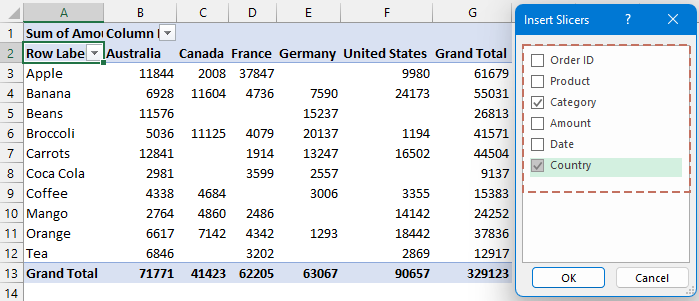
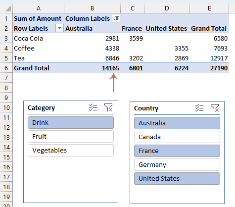
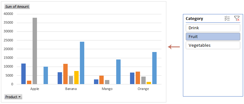
- The slicers for the selected fields are created. Click on any of the slicer buttons to filter the data in the PivotTable. In this example, I will filter for Drink from Australia, France, or the United States. See screenshot:


- To filter by multiple items, either hold down the Ctrl key and click on the items you want to filter, or click the Multi-Select button
 to enable multiple selection.
 - To reset or clear the filters in a slicer, click on the Clear Filter button
 in the slicer.
 to enable multiple selection.
 in the slicer.
Insert and use slicer in Excel table
Inserting and using a slicer in an Excel table can significantly enhance the data interaction and analysis experience. Here’s how you can optimize this process:
- Click anywhere inside your Excel table.
Note: Ensure your data is organized in an Excel table. If it’s not, select your data range, then go to the "Insert" tab on the ribbon and click on "Table". Make sure to check the box for "My table has headers" if your data includes headers.
- Navigate to the "Table Design" tab on the ribbon in Excel 2021 and 365. See screenshot:Tips: In other Excel versions, please do as this:
In Excel 2013-2019, under the "Design" tab, and then click "Insert Slicer".
In Excel 2010, it is not possible to insert slicers in tables.
- In the "Insert Slicers" dialog box, select the checkbox next to each field you want to add a slicer for, then click OK.
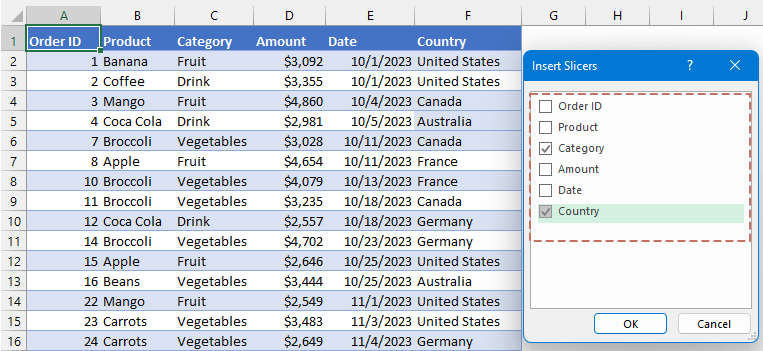
- The slicers for the selected fields are created. Click on any of the slicer buttons to filter the data in the table. In this example, I will filter for Fruit from Germany. See screenshot:


- To filter by multiple items, either hold down the Ctrl key and click on the items you want to filter, or click the Multi-Select button to enable multiple selection.
- To reset or clear the filters in a slicer, click on the Clear Filter button in the slicer.
Create and use slicer in Pivot Chart
Creating and using a slicer in a Pivot Chart in Excel not only enhances the interactivity of your data presentation but also allows for dynamic analysis. Here's a detailed guide on how to optimize this process:
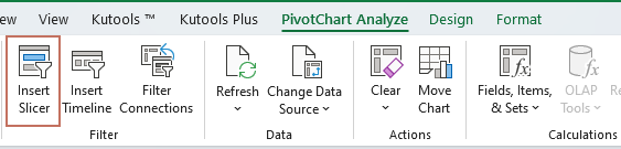
- Create a Pivot Chart first. And then, click to select the Pivot Chart.
- Go to the "PivotChart Analyze" tab, and click "Insert Slicer". See screenshot:Tips: In Excel 2010-2019, under the "Analyze" tab, click "Insert Slicer".
- In the "Insert Slicers" dialog box, select the checkbox next to each field you want to add a slicer for, then click OK.

- Now, the slicer is created at once. Click the buttons on the slicer to filter the data displayed in your Pivot Chart. The chart will update immediately to reflect only the data related to your slicer selections.


- To filter by multiple items, either hold down the Ctrl key and click on the items you want to filter, or click the Multi-Select button to enable multiple selection.
- To reset or clear the filters in a slicer, click on the Clear Filter button in the slicer.
- If desired, you can integrate the slicer box into the chart area. To do this, enlarge the chart area and reduce the plot area by dragging their edges. Then, move the slicer box into the newly created space. See the demo below:


How to connect slicer to multiple pivot tables / pivot charts?
Connecting a slicer to multiple PivotTables or Pivot Charts in Excel allows for synchronized filtering across various data representations, enhancing the comprehensiveness and interactivity of your data analysis. This section explains how to connect a slicer to multiple PivotTables or Pivot Charts.
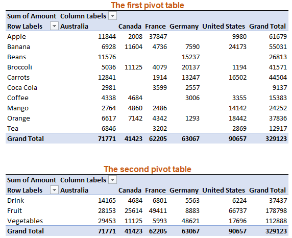
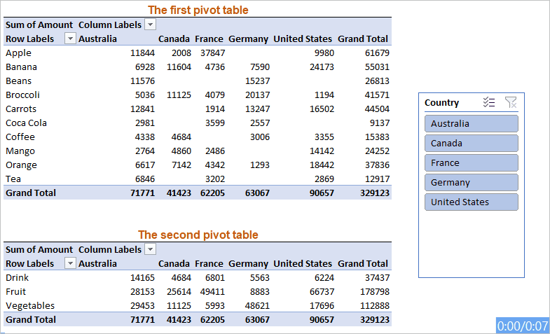
- Create two or more PivotTables or Pivot Charts, in the same sheet. See screenshot:
Note: A slicer can only be linked to pivot tables and pivot charts that share the same data source. Thus, it is essential to create these pivot tables and pivot charts from the same dataset.
- Then, create a slicer for any PivotTable or Pivot Chart by following the steps outlined in the Create Slicer for PivotTable or Pivot Chart section.
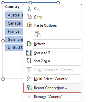
- After creating the slicer, right click it, then choose "Report Connections" ("PivotTable Connections" in Excel 2010). See screenshot:
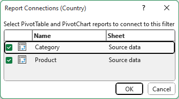
- You’ll see a list of all the PivotTables in the workbook that are based on the same data source. Check the boxes next to the PivotTables you want to connect with the slicer. And then, click OK. See screenshot:
- From now on, you can apply filters to all connected PivotTables by simply clicking a button on the slicer. See the demo below:


- To filter by multiple items, either hold down the Ctrl key and click on the items you want to filter, or click the Multi-Select button to enable multiple selection.
- To reset or clear the filters in a slicer, click on the Clear Filter button in the slicer.
Format slicers in Excel
Formatting slicers in Excel helps make your reports look better and easier to use. You can change how slicers look, resize them, organize their layout, adjust their settings, and fix their position on the sheet. Let's explore how to do these to make your Excel slicers work better and look great.
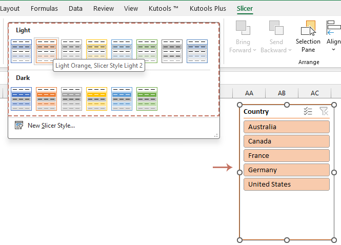
Change slicer style
- Click on the slicer to activate the "Slicer Tools Options" (Excel 2010-2019) or "Slicer" (Excel 2021, 365) tab in the ribbon.
- Navigate to the "Options" tab or "Slicer" tab. Then, pick a style from the "Slicer Styles" group to change the appearance of your slicer, see screenshot:

Resize slicers
● Resize the slicer box:
Normally, you can change the slicer's size is by dragging the edges or the corner of the box. See the demo below:
● Resize slicer buttons:
Click to select the slicer, and then go to the "Slicer Tools Options" (Excel 2010-2019) or "Slicer" (Excel 2021, 365) tab in the ribbon. Under the "Buttons" group, adjust the number of the "Height" or "Width" in the slicer to your need. See screenshot:
● Adjust the number of columns in slicer:
When a slicer in Excel contains too many items to fit within its box, you can arrange these items across multiple columns to ensure they are all visible and accessible. This will help in making all slicer items visible and ensures that users can easily interact with the slicer without having to scroll up and down.
Click to select the slicer, and then go to the "Slicer Tools Options" (Excel 2010-2019) or "Slicer" (Excel 2021, 365) tab in the ribbon. Under the "Buttons" group, adjust the number of columns in the slicer to your need. See screenshot:
Change the slicer settings
To change the slicer settings in Excel, follow these steps to customize its behavior and appearance according to your needs:
Click on the slicer you want to modify, right-click it and choose "Slicer Settings", in the "Slicer Setting" dialog box you can set the following operations:
- Name and Caption: Change the name or caption of the slicer for better identification. If you want to hide the slicer header, uncheck the "Display header" checkbox;
- Sorting: Choose how to sort the items in the slicer, in ascending or descending order.
- Filtering Options: Choose to hide items with no data or those deleted from the data source to keep the slicer clean and relevant.
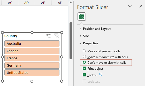
Lock the slicer position in a worksheet
Locking a slicer ensures it stays fixed at a certain spot on the worksheet, avoiding any unintended movement when rows and columns are added or deleted, PivotTable fields are modified, or other alterations are made to the sheet. To secure a slicer's position on a worksheet, follow these steps:
- Right-click the slicer, and choose "Size and Properties" from the context menu.

- In the "Format Slicer" pane, under "Properties", select the "Don't move or size with cells" option. See screenshot:


Disconnect a slicer
Disconnecting a slicer in Excel is useful when you need to unlink it from a PivotTable or PivotChart, allowing for independent data analysis without affecting other linked elements.
- Click anywhere in the PivotTable to which slicer you want to disconnect.
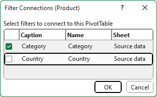
- Then, navigate to "PivotTable Analyze" tab (Excel 2021, Excel 365) or "Analyze" (Excel 2013-2019), and click "Filter Connections". See screenshot:

- In the "Filter Connections" dialog box, uncheck the check box of the slicer you want to disconnect, and click OK.


Delete a slicer
To permanently remove a slicer from your worksheet, you can use either of the following methods:
- Click on the slicer to select it and then press the Delete key.
- Right-click on the slicer and choose Remove (Slicer Name) from the context menu.
Benefits of using slicers in Excel
Using slicers in Excel offers several benefits that enhance data analysis and presentation:
- Enhanced Interactivity:
- Slicers provide a user-friendly interface that makes it easier for users to interact with the data. They can quickly filter and segment the data without navigating complex menus or dialogs.
- Improved Data Visualization:
- By allowing users to filter through data and view only what is relevant, slicers help in creating dynamic and interactive charts and tables that better represent the underlying data trends and patterns.
- Enhance Data Security:
- Slicers enhance data security and integrity by enabling users to filter the required information without modifying the actual dataset, ensuring the original data remains unaltered and reliable.
In conclusion, slicers provide a dynamic and intuitive method for filtering and analyzing data in Excel, making them a powerful tool for data analysis and presentation. If you're interested in exploring more Excel tips and tricks, our website offers thousands of tutorials, please click here to access them. Thank you for reading, and we look forward to providing you with more helpful information in the future!
Related Articles:
- Count unique values in pivot table
- By default, when we create a pivot table based on a range of data which contains some duplicate values, all the records will be counted as well, but, sometimes, we just want to count the unique values based on one column to get the right screenshot result. In this article, I will talk about how to count the unique values in pivot table.
- Reverse a pivot table in Excel
- Have you ever wanted to reverse or transpose the pivot table in Excel just like the below screenshots shown. Now I will tell you the quick ways to reverse a pivot table in Excel.
- Change multiple field settings in pivot table
- When you create a pivot table in a worksheet, after dragging the fields to the Values list in the PivotTable Field List, you may get all the same Count function as following screenshot shown. But now, you want the Sum of function to replace the Count of function at once, how could you change the calculation of multiple pivot table fields at once in Excel?
- Add multiple fields into pivot table
- When we create a pivot table, we need to drag the fields into the Row Labels or Values manually one by one. If we have a long list of fields, we can add a few row labels quickly, but the remaining fields should be added to the Value area. Are there any quick methods for us to add all the other fields into the Value area with one click in the pivot table?
Table of contents
- What are Slicers in Excel?
- How to add and use slicer in Excel?
- Add and use slicer in PivotTable
- Insert and use slicer in Excel table
- Create and use slicer in Pivot Chart
- Connect slicer to multiple PivotTables / Pivot Charts
- Format slicers in Excel
- Change slicer style
- Resize a slicer
- Change the slicer settings
- Lock the slicer position
- Disconnect a slicer
- Delete a slicer
- Benefits of using slicers in Excel
- Related Articles
- The Best Office Productivity Tools
- Comments
Best Office Productivity Tools
Supercharge Your Excel Skills with Kutools for Excel, and Experience Efficiency Like Never Before. Kutools for Excel Offers Over 300 Advanced Features to Boost Productivity and Save Time. Click Here to Get The Feature You Need The Most...
Office Tab Brings Tabbed interface to Office, and Make Your Work Much Easier
- Enable tabbed editing and reading in Word, Excel, PowerPoint, Publisher, Access, Visio and Project.
- Open and create multiple documents in new tabs of the same window, rather than in new windows.
- Increases your productivity by 50%, and reduces hundreds of mouse clicks for you every day!
All Kutools add-ins. One installer
Kutools for Office suite bundles add-ins for Excel, Word, Outlook & PowerPoint plus Office Tab Pro, which is ideal for teams working across Office apps.
- All-in-one suite — Excel, Word, Outlook & PowerPoint add-ins + Office Tab Pro
- One installer, one license — set up in minutes (MSI-ready)
- Works better together — streamlined productivity across Office apps
- 30-day full-featured trial — no registration, no credit card
- Best value — save vs buying individual add-in