How to create multi level dependent drop down list in Excel?
Drop-down lists in Excel are a powerful tool for data entry, ensuring consistency and reducing errors. However, when you need to create multi-level dependent drop-down lists—where the options in each subsequent list depend on the selection made in the previous one—things can get more complex. This guide will walk you through the process step-by-step, with tips for optimization and best practices.
Create multi-level dependent drop down list in Excel
To create a multi-level dependent drop down list, please do with the following steps:
Step1: create the data for the multi-level dependent drop down list.
1. First, create the first, second and third drop down list data as below screenshot shown:

Step2: create range names for each drop down list values.
2. Then, select the first drop down list values (excluding the header cell), and then give a range name for them in the "Name box" which besides the formula bar, see screenshot:

3. And then, select the second drop down list data and then click "Formulas" > "Create from Selection", see screenshot:

4. In the popped out "Create Names from Selection" dialog box, check only "Top row" option, see screenshot:

5. Click "OK", And the range names have been created for each second drop down data at once, then, you should create range names for the third drop down list values, go on clicking "Formulas" > "Create from Selection", in the "Create Names from Selection" dialog box, check only "Top row" option, see screenshot:

6. Then, click "OK" button, the third level drop down list values have been defined range names.
- Tips: You can go the "Name Manager" dialog box to see all the created range names which have been located into the "Name Manager" dialog box as below screenshot shown:


Step3: create Data Validation drop down list.
7. And then, click a cell where you want to put the first dependent drop down list, for example, I will select cell I2, then, click "Data" > "Data Validation" > "Data Validation", see screenshot:

8. In the "Data Validation" dialog box, under the "Settings" tab, choose "List" from the "Allow" drop down list, and then enter the following formula into the "Source" text box.
=ContinentsNote: In this formula, "Continents" is the range name of the first drop down values you created in step 2, please change it to your need.

9. Then, click "OK" button, the first drop down list has been created as below screenshot shown:

10. And then, you should create the second dependent drop down, please select a cell where you want to put the second drop down list, here, I will click J2, and then go on clicking "Data" > "Data Validation" > "Data Validation", in the "Data Validation" dialog box, do the following operations:
- (1.) Choose List from the "Allow" drop down list;
- (2.) Then enter this formula into the "Source" text box.
=INDIRECT(SUBSTITUTE(I2," ","_"))
Note: In the above formula, I2 is the cell which contains the first drop down list value, please change it to your own.

11. Click "OK", and the second dependent drop down list has been created at once, see screenshot:

12. In this step, you should create the third dependent drop down list, click a cell to output the third drop down list value, here, I will select cell K2, and then click "Data" > "Data Validation" > "Data Validation", in the "Data Validation" dialog box, do the following operations:
- (1.) Choose "List" from the "Allow" drop down list;
- (2.) Then enter this formula into the "Source" text box.
=INDIRECT(SUBSTITUTE(J2," ","_"))
Note: In the above formula, J2 is the cell which contains the second drop down list value, please change it to your own.

13. Then, click "OK", and the three dependent drop down list has been created successfully, see the below demo:

Create multi-level dependent drop down list in Excel with an amazing feature
Creating multi-level dependent drop-down lists in Excel can be tricky, especially when dealing with large datasets or complex hierarchies. "Kutools for Excel" eliminates the hassle by offering a user-friendly interface and advanced features that simplify the process. With Kutools’ "Dynamic Drop-down List", you can create dynamic, multi-level dependent drop-down lists in just a few clicks—no advanced Excel skills required.
1. First, you should create your data in the format shown in the screenshot below:

2. Then, click "Kutools" > "Drop-down List" > "Dynamic Drop-down List", see screenshot:

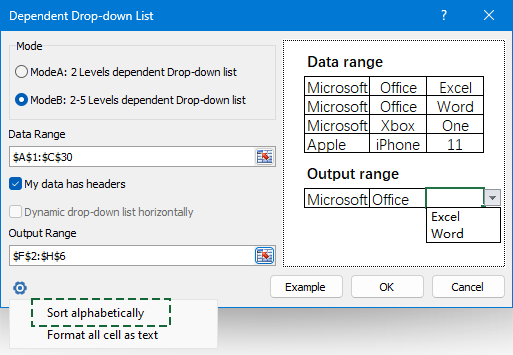
3. In the "Dependent Drop-down List" dialog box, please do the following operations:
- Check the "3-5 Levels dependent Drop-down list" option in the "Typ"e section;
- Specify the data range and output range as you need.
- Then, click "OK" button.


4. Now, the 3-level drop down list has been created as the following demo shown:
Creating multi-level dependent drop-down lists in Excel doesn’t have to be complicated. By following the steps above or using Kutools for Excel, you can streamline your data entry process, reduce errors, and improve efficiency. Whether you’re managing small datasets or complex hierarchies, these techniques will help you take your Excel skills to the next level. If you're interested in exploring more Excel tips and tricks, our website offers thousands of tutorials.
More relative drop down list articles:
- Auto Populate Other Cells When Selecting Values In Excel Drop Down List
- Let’s say you have created a drop down list based on the values in cell range B8:B14. When you selecting any value in the drop down list, you want the corresponding values in cell range C8:C14 be automatically populated in a selected cell. For example, when you select Lucy in the drop down list, it will auto populate a score 88 in cell D16.
- Create A Dependent Drop Down List In Google Sheet
- Inserting normal drop down list in Google sheet may be an easy job for you, but, sometimes, you may need to insert a dependent drop down list which means the second drop down list depending on the choice of the first drop down list. How could you deal with this task in Google sheet?
- Create Drop Down List With Images In Excel
- In Excel, we can quickly and easily create a drop down list with cell values, but, have you ever tried to create a drop down list with images, that is to say, when you click one value from the drop down list, its relative image will be displayed at the same time. In this article, I will talk about how to insert a drop down list with images in Excel.
- Select Multiple Items From Drop Down List Into A Cell In Excel
- The drop-down list is frequently used in the Excel daily work. By default, only one item can be selected in a drop-down list. But in some times, you may need to select multiple items from the drop down list into one single cell as below screenshot shown. How can you handle it in Excel?
- Create Drop Down List With Hyperlinks In Excel
- In Excel, adding drop down list may help us to solve our work efficiently and easily, but, have you ever tried to create drop down list with hyperlinks, when you choose the URL address from the drop down list, it will be open the hyperlink automatically? This article, I will talk about how to create drop down list with activated hyperlinks in Excel.
Best Office Productivity Tools
Supercharge Your Excel Skills with Kutools for Excel, and Experience Efficiency Like Never Before. Kutools for Excel Offers Over 300 Advanced Features to Boost Productivity and Save Time. Click Here to Get The Feature You Need The Most...
Office Tab Brings Tabbed interface to Office, and Make Your Work Much Easier
- Enable tabbed editing and reading in Word, Excel, PowerPoint, Publisher, Access, Visio and Project.
- Open and create multiple documents in new tabs of the same window, rather than in new windows.
- Increases your productivity by 50%, and reduces hundreds of mouse clicks for you every day!
All Kutools add-ins. One installer
Kutools for Office suite bundles add-ins for Excel, Word, Outlook & PowerPoint plus Office Tab Pro, which is ideal for teams working across Office apps.
- All-in-one suite — Excel, Word, Outlook & PowerPoint add-ins + Office Tab Pro
- One installer, one license — set up in minutes (MSI-ready)
- Works better together — streamlined productivity across Office apps
- 30-day full-featured trial — no registration, no credit card
- Best value — save vs buying individual add-in