How to list column header names in Excel?
Navigating a large Excel spreadsheet with numerous columns that overflow across multiple pages can be cumbersome, especially when you need to scroll back and forth to view and locate specific column header names. If you're looking for an easier way to access and organize these headers, there are several efficient techniques you can employ. This guide will show you simple tricks to quickly list and identify all column header names in your Excel spreadsheet, enhancing your data management efficiency.
- List column header names with the Paste Special command
- List and locate column header names with Kutools for Excel
- List column header names with Excel formulas
- List column header names with VBA code
List column header names with the Paste Special command
The built-in "Paste Special" command in Excel allows you to transpose a row into a column, making it simple to view all your column headers at a glance without the need to scroll horizontally through wide tables. This approach is particularly helpful when you need to visually reference all headers side-by-side or prepare a summary of your data structure for documentation purposes.
- Select the row containing your column header names. Typically, this is the first row (Row1) of your worksheet.
- Copy the selected row. You can do this by pressing Ctrl+C or right-clicking and selecting Copy.
- Locate a blank area on your worksheet where you want to display the headers in a column. Right-click in your desired cell and choose Paste Special, then click the Transpose button.
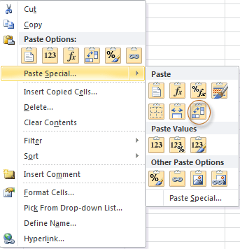

All your column header names will now appear as a vertical list, each in its own cell within a single column. This method makes it easier to scan and review headers without scrolling horizontally. See screenshot:
 |
 |
While this method provides a convenient way to quickly list column header names, it does not offer automatic updates if your headers change, nor does it assist with locating columns within your worksheet efficiently.
List and locate column header names with Kutools for Excel
For users seeking a more advanced method to manage and interact with column headers, Kutools for Excel offers a dedicated feature within its Navigation Pane. Not only can you view all column headers at a glance, but you can also instantly jump to any column, streamlining your workflow—particularly useful in worksheets with dozens or even hundreds of columns.
After installing Kutools for Excel, select Kutools > Navigation to open the Navigation pane.
Within the "Column List" section, the headers of the current worksheet are automatically listed in order. Simply click on any column name to instantly jump to that column on your worksheet. This saves time and ensures accuracy when working with expansive data sets or when collaborating with colleagues who may not be familiar with your spreadsheet structure.
To explore this feature in more detail, please visit the following article: Navigation Pane – List Sheets, Workbooks, Columns, Names and insert auto text in Excel
Kutools for Excel - Supercharge Excel with over 300 essential tools, making your work faster and easier, and take advantage of AI features for smarter data processing and productivity. Get It Now
List column header names with Excel formulas
For users who prefer a dynamic, formula-based solution, Excel's built-in functions, such as INDEX and FILTER enable you to display or extract column header names automatically. These methods are especially beneficial in scenarios where your header row may change over time, and you want a list that updates immediately when new headers are added or existing ones modified.
Using INDEX with COLUMN:
This method allows you to quickly list header names from the first row into a column. It works well for standard tables where headers are in Row1.
1. Enter the following formula in a blank cell where you want the first header listed (for example, in cell B2):
=INDEX($1:$1, ROW(A1))2. Press Enter to display the first header. Then, drag the formula down to subsequent cells (B3, B4, etc.) to list each header in order. Each copied formula will reference the next column header in Row 1.
Tip: If your headers start in a different row, adjust $1:$1 to match, and if listing headers from a specific range rather than the entire row, modify the formula range accordingly. Make sure there are no blank columns in your header row; otherwise, formula results may be empty.
Dynamic extraction with FILTER (Excel 365, Excel 2021):
To display unique header names or filter specific headers from a table, you can use a formula like:
=TRANSPOSE(FILTER(1:1,1:1<>""))This will list all non-blank header cells from Row 1 vertically in your chosen range. Input the formula in a blank column and press Enter; the result spills over adjacent cells automatically. Useful when working with tables containing optional header fields or dynamic column structures.
Error reminder: The FILTER function is available only in Excel 365 and Excel 2021. If you experience any errors, verify your Excel version supports dynamic array formulas.
If you have merged header cells or use complex header arrangements, formula accuracy may be affected. For cleaner results, ensure your headers are in a single row without merged cells.
Excel formula methods enable automatic updates, providing flexibility in your workflow. However, for very large tables, performance may slightly decrease due to formula calculation overhead.
List column header names with VBA code
If you frequently need to create a list of column header names or want to automate the process, writing a simple VBA macro can help. This solution is particularly suitable for advanced users or those working with large, frequently changing spreadsheets. VBA macros can output the list anywhere you choose—on a new worksheet, in a specific range, or even as part of a report workflow.
To create a header name listing macro, follow these steps:
1. Activate the sheet that you want to list all column header names. and then click Developer Tools > Visual Basic. In the Microsoft Visual Basic for Applications window that appears, click Insert > Module. Then copy and paste the code below into the new module:
Sub ListHeaders()
    Dim ws As Worksheet
    Dim outputWs As Worksheet
    Dim lastCol As Long
    Dim i As Long

    On Error Resume Next
    xTitleId = "KutoolsforExcel"

    Set ws = Application.ActiveSheet
    Set outputWs = Worksheets.Add
    outputWs.Name = "HeaderList"

    lastCol = ws.Cells(1, ws.Columns.Count).End(xlToLeft).Column

    For i = 1 To lastCol
        outputWs.Cells(i, 1).Value = ws.Cells(1, i).Value
    Next i
End Sub2. Click the ![]() button to run the code. A new worksheet named HeaderList will be created, and all column header names from the first row of your active sheet will be listed vertically.
button to run the code. A new worksheet named HeaderList will be created, and all column header names from the first row of your active sheet will be listed vertically.
Practical tips:
- If you prefer output in the same worksheet, adjust
outputWs = wsand modify the target output cell accordingly. - This macro automatically detects the last used column in Row 1. Avoid placing headers outside the first row or having merged header cells for best results.
- Running the macro repeatedly will create new worksheets each time. Rename or delete previous sheets as needed to avoid confusion.
Troubleshooting:
- If you encounter an error due to worksheet naming conflicts, the macro may not run. Delete or rename any existing "HeaderList" worksheet before running again.
- Save your work before executing VBA macros to prevent unintentional loss of data through automation.
When deciding which method to use for listing column header names in Excel, consider the structure of your dataset, how frequently headers might change, and whether manual or automated updates are more suitable. For quick, manual listing, Excel’s "Paste Special" approach works well; for ongoing, interactive management, Kutools provides user-friendly navigation. Formula methods are best for smaller tables or where dynamic updates are desired, while VBA automates listing for large or regularly updated workbooks. If you experience issues such as blank outputs or formula errors, check your data layout (no merged cells, headers in row 1) and ensure compatibility with your Excel version. These solutions collectively enhance the clarity and efficiency of managing complex spreadsheets.
Related Articles
- List all worksheets in one workbook
- Navigate between windows in Workbooks
- Show navigation pane
- Navigate between cells
- List named ranges
Best Office Productivity Tools
Supercharge Your Excel Skills with Kutools for Excel, and Experience Efficiency Like Never Before. Kutools for Excel Offers Over 300 Advanced Features to Boost Productivity and Save Time. Click Here to Get The Feature You Need The Most...
Office Tab Brings Tabbed interface to Office, and Make Your Work Much Easier
- Enable tabbed editing and reading in Word, Excel, PowerPoint, Publisher, Access, Visio and Project.
- Open and create multiple documents in new tabs of the same window, rather than in new windows.
- Increases your productivity by 50%, and reduces hundreds of mouse clicks for you every day!
All Kutools add-ins. One installer
Kutools for Office suite bundles add-ins for Excel, Word, Outlook & PowerPoint plus Office Tab Pro, which is ideal for teams working across Office apps.
- All-in-one suite — Excel, Word, Outlook & PowerPoint add-ins + Office Tab Pro
- One installer, one license — set up in minutes (MSI-ready)
- Works better together — streamlined productivity across Office apps
- 30-day full-featured trial — no registration, no credit card
- Best value — save vs buying individual add-in