How to highlight row if cell contains text/value/blank in Excel?
In Excel, it's often necessary to quickly identify and visually highlight rows based on specific criteria—such as whether a cell contains a particular text, value, or remains blank. Highlighting entire rows where certain conditions are met can significantly enhance readability and data analysis, making it easier to spot relevant information at a glance and act upon it efficiently.
The following methods provide practical solutions suited for different scenarios and requirements. You may choose Conditional Formatting for standard rules, Kutools for Excel features for interactive selection, or advanced VBA code for more dynamic or complex criteria.
Highlight entire row if cell contains specific text/value/blank with Conditional Formatting
Highlight entire row if cell contains specific text/value with Kutools for Excel
Highlight entire row if cell contains specific text/value/blank with VBA Code
Highlight entire row if cell contains one of specific values in another column
Highlight row if cell contains specific text/value/blank with Conditional Formatting
Conditional Formatting is a built-in Excel feature designed to format cells or rows automatically based on predefined rules. It’s ideal for scenarios where you want the formatting to update dynamically whenever data changes. This method works best for simple conditions like checking if a cell equals a particular value, contains certain text, or is blank.
To highlight entire rows in your table where a cell contains specific text, a specific value, or is blank, follow these steps:
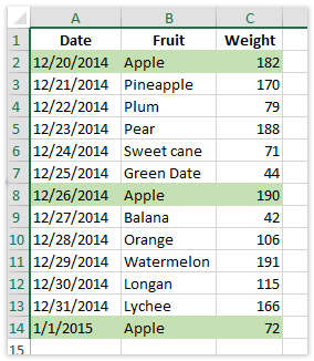
1. Select the purchase table, excluding column headings. Ensure you only select the relevant range—starting from the first data row to the last—to avoid formatting header cells.
2. Go to the "Home" tab, then click "Conditional Formatting" > "New Rule". See the screenshot below:
3. In the New Formatting Rule dialog box, configure your rule as shown in the screenshot:
(1) Choose "Use a formula to determine which cells to format" under "Select a Rule Type".
(2) In the "Format values where this formula is true" box, enter the formula that matches your criteria:
=$B2="Apple"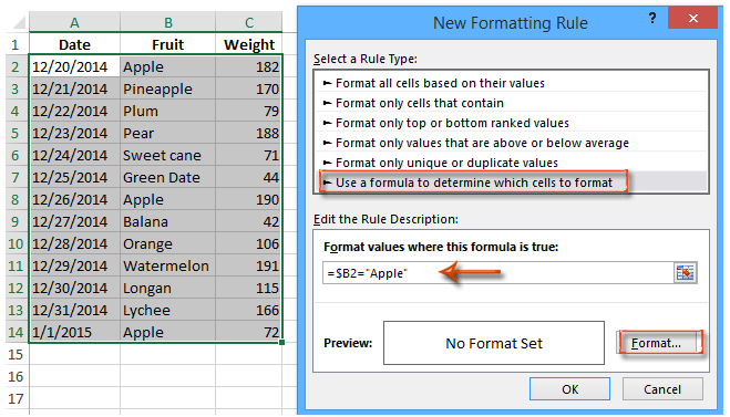
Notes:
- The formula
=$B2="Apple"checks whether cell B of each row exactly matches the text "Apple". Adjust$B2to the actual column you want to base the condition on, and update "Apple" to your target value. - To highlight rows where the cell is blank, use
=$B2="". - If you want to highlight rows where the cell starts with specific text, you can use
=LEFT($B2,5)="Apple", and similarly use=RIGHT($B2,5)="Apple"for cells ending with that text. - Conditional Formatting formulas are case-insensitive by default. For case-sensitive matching, use
=EXACT($B2,"Apple").
4. In the Format Cells dialog box, switch to the "Fill" tab, choose your highlight color, and click "OK".
5. Press "OK" again to close the New Formatting Rule dialog box.
After completing these steps, all rows in your selected range that match the specified condition will be highlighted accordingly. If you edit the values later, the highlighting will update automatically.
Practical Tips: Conditional Formatting allows for multiple rules. You can stack different criteria to highlight rows with different colors based on various conditions. If the rule does not appear to work, double-check the range selection and formula reference style. To remove formatting, use "Clear Rules" in the Conditional Formatting menu.
Pros: Dynamic, updates with cell changes, no add-in required.
Cons: Not ideal for very complex or multifaceted criteria, may slow down large files.
Highlight row if cell contains specific text/value with Kutools for Excel
Kutools for Excel provides a user-friendly way to enhance data selection and formatting in tables. The "Select Specific Cells" feature enables users to quickly select rows based on criteria such as cells containing certain text or values, then manually apply highlight colors.
1. Select the column to search for the specific text or value. Ensure selection starts from the first relevant cell, and includes all entries you wish to check.
2. Click "Kutools" > "Select" > "Select Specific Cells".
3. In the Select Specific Cells dialog box (see above screenshot):
(1) Check "Entire row" under "Selection type".
(2) In "Specific Type", set the drop-down to "Contains", and enter your target text.
(3) Click "OK".
4. In the follow-up dialog, confirm by clicking "OK". At this stage, all relevant rows will be selected automatically.

5. Return to the "Home" tab, click "Fill Color", and choose a highlight shade from the drop-down to format your selected rows.
Kutools ensures that users can rapidly identify and color-code data without writing formulas or navigating complex menus. This method is especially effective for one-time selection and formatting of specific rows, rather than ongoing rule-driven highlighting.
Practical Tips: After using Kutools, you can use Excel's sorting or filtering functions to work only with highlighted rows. Remember to check the selected rows before applying fill color, as unintentional selection can overwrite existing formatting.
Pros: Quick, interactive, no formulas needed, handles a wide range of criteria with built-in logic.
Cons: Not dynamic—new data will need the process repeated; requires Kutools for Excel installed.
Kutools for Excel - Supercharge Excel with over 300 essential tools, making your work faster and easier, and take advantage of AI features for smarter data processing and productivity. Get It Now
Highlight entire row if cell contains specific text/value/blank with VBA Code
For users who require more advanced or dynamic criteria beyond the scope of Conditional Formatting or Kutools, VBA (Visual Basic for Applications) provides a way to automate row highlighting. This method is especially helpful when you want to highlight rows based on several different rules (such as containing any value from a list, handling multiple columns, or matching complex patterns) and have the formatting done instantly upon running the code.
Preparation: Save your workbook before running VBA and make sure you know which column and row range to target. VBA changes are immediate and may be difficult to undo without an original backup.
1. Open the VBA Editor by clicking Developer Tools > Visual Basic. In the Microsoft Visual Basic for Applications window that appears, click Insert > Module, and copy-paste the following code into the module:
Sub HighlightRowsByCellContent()
    Dim ws As Worksheet
    Dim rng As Range
    Dim lastRow As Long
    Dim targetCol As String
    Dim searchValue As String
    Dim cell As Range
    Dim xTitleId As String
    Dim i As Long

    On Error Resume Next
    Set ws = Application.ActiveSheet
    xTitleId = "KutoolsforExcel"

    ' Prompt for the target column by letter (e.g., "B") and the value to search for
    targetCol = Application.InputBox("Enter the column letter to check (e.g., B):", xTitleId, "B", Type:=2)
    searchValue = Application.InputBox("Enter the text/value to search for (leave blank to find blank cells):", xTitleId, "", Type:=2)

    lastRow = ws.Cells(ws.Rows.Count, targetCol).End(xlUp).Row

    ' Loop through each row and highlight if criteria match
    For i = 2 To lastRow
        Set cell = ws.Cells(i, Columns(targetCol).Column)
        If searchValue = "" Then
            If Trim(cell.Value) = "" Then
                ws.Rows(i).Interior.Color = vbYellow
            End If
        Else
            If InStr(1, cell.Value, searchValue, vbTextCompare) > 0 Then
                ws.Rows(i).Interior.Color = vbYellow
            End If
        End If
    Next i
End Sub
2. To run the code, press ![]() (the Run button) in the VBA window. A prompt will let you specify the target column and the value (or leave the value blank for blank cell matching). All matching rows in the active worksheet will be highlighted in yellow.
(the Run button) in the VBA window. A prompt will let you specify the target column and the value (or leave the value blank for blank cell matching). All matching rows in the active worksheet will be highlighted in yellow.
Parameter explanations and advanced options:
- targetCol: Enter the column letter you want to check (for example, "B" checks column B for each row).
- searchValue: Enter the text or value you wish to find. To find blank cells, leave this box empty.
- Interior.Color: The code uses yellow as the highlight color. You can change
vbYellowtovbGreen,vbCyan, or useRGB(r,g,b)for custom colors.
Tips and Precautions:
- Always save your workbook before running macros as formatting is instantly applied.
- If you want to clear highlighting later, run a similar macro setting
ws.Rows(i).Interior.ColorIndex = xlNone. - This VBA operates on the active worksheet. For other sheets, adjust
Set ws = Worksheets("SheetName"). - For large datasets, the process may take a few seconds.
Troubleshooting: If the code does not highlight rows, check these possible causes:
- Incorrect column letter – always enter the letter, not the column number.
- Row numbers must start from your data table (the example starts at row2, assuming row1 is headers).
Pros: Highly flexible, supports complex criteria and can be modified for advanced scenarios.
Cons: Requires some familiarity with VBA and can overwrite manual formatting.
Highlight entire row if cell contains one of specific values in another column
Some situations demand highlighting rows only when a cell matches any value from a list in another column. For example, you might have a column of product names and want to automatically highlight all rows where the product matches any name from a specified list. Kutools for Excel's "Compare Ranges" utility offers a streamlined way to accomplish this without complex formulas.
1. Go to "Kutools" > "Select > Select Same & Different Cells".
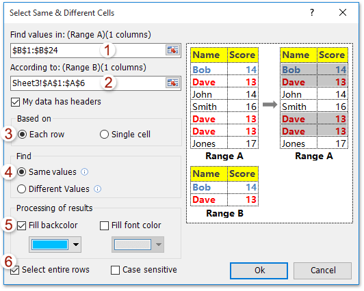
2. In the Select Same & Different Cells dialog, configure as follows:
- In "Find values in", specify the column that you want to examine for the match.
- In "According to", choose the column containing your list of specific values.
- Check "Each row" under "Based on".
- Select "Same Values" under "Find".
- Enable "Fill backcolor" under "Processing of results" and select a color.
- Ensure "Select entire rows" is checked.
3. Click "OK" to run the utility. A notification will show how many rows were matched and highlighted. Click "OK" to close.
As a result, your table will display highlighted rows wherever the specified cell matches one of the values in your reference column.
This technique is particularly useful for cross-referencing data between lists—such as matching product codes with a list of active inventory or identifying all transactions linked to a customer group.
Tips: If your value lists are large, use Excel's "Remove Duplicates" to clean up before running the comparison. Double-check both columns for extraneous spaces or differences that can affect results. Formatting will not automatically update if data changes—you'll need to run the process again.
Pros: Effective for cross-list matching, supports batch row selection and highlighting.
Cons: Requires Kutools add-in, is not automatic—rerun if data changes.
Kutools for Excel - Supercharge Excel with over 300 essential tools, making your work faster and easier, and take advantage of AI features for smarter data processing and productivity. Get It Now
Demo: highlight row if cell contains certain value or one of specified values
Related Articles
How to prevent saving if specific cell is blank in Excel?
How to not calculate (ignore formula) if cell is blank in Excel?
How to use IF function with AND, OR, and NOT in Excel?
How to display warning/alert messages if cells are blank in Excel?
How to enter/display text or message if cells are blank in Excel?
How to delete rows if cells are blank in a long list in Excel?
Best Office Productivity Tools
Supercharge Your Excel Skills with Kutools for Excel, and Experience Efficiency Like Never Before. Kutools for Excel Offers Over 300 Advanced Features to Boost Productivity and Save Time. Click Here to Get The Feature You Need The Most...
Office Tab Brings Tabbed interface to Office, and Make Your Work Much Easier
- Enable tabbed editing and reading in Word, Excel, PowerPoint, Publisher, Access, Visio and Project.
- Open and create multiple documents in new tabs of the same window, rather than in new windows.
- Increases your productivity by 50%, and reduces hundreds of mouse clicks for you every day!
All Kutools add-ins. One installer
Kutools for Office suite bundles add-ins for Excel, Word, Outlook & PowerPoint plus Office Tab Pro, which is ideal for teams working across Office apps.
- All-in-one suite — Excel, Word, Outlook & PowerPoint add-ins + Office Tab Pro
- One installer, one license — set up in minutes (MSI-ready)
- Works better together — streamlined productivity across Office apps
- 30-day full-featured trial — no registration, no credit card
- Best value — save vs buying individual add-in