Excel REPT function
In Excel, the REPT function is used to repeat the characters a specified number of times. It is a useful function which can help you to deal with many cases in Excel, such as padding cells to a certain length, creating in-cell bar chart, and so on.
- Example 1: Using the REPT function to repeat characters multiple times
- Example 2: Using the REPT function to pad leading zeros to make the text same length
- Example 3: Using the REPT function to create in-cell bar chart
Syntax:
The syntax for the REPT function in Excel is:
Arguments:
- text: Required. The text that you want to repeat.
- number_times: Required. The number of times to repeat the text, it must be a positive number.
Notes:
- 1. If the result of the REPT function is more than 32,767 characters, an #VALUE! error value will display.
- 2. If number_times is 0, the REPT function returns empty text.
- 3. If number_times is not an integer, it is truncated. For example, if the number_times is 6.8, it will repeat the text 6 number of times only.
Return:
Return the repeated text by specific number of times.
Examples:
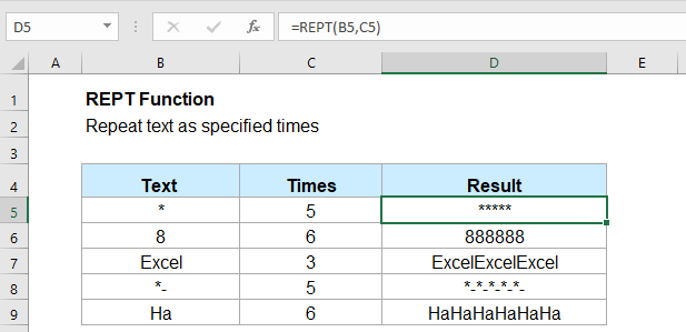
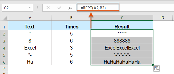
Example 1: Using the REPT function to repeat characters multiple times
Please use this REPT function to repeat the characters x times:
And, you will get the result as you need, see screenshot:
Example 2: Using the REPT function to pad leading zeros to make the text same length
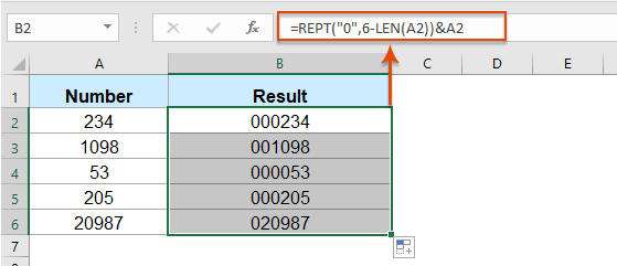
Supposing, you have a list of number with different lengths, now, you want to make all the numbers of the same length (6-digit). In this case, you can pad the leading zeros in front of the numbers by using the REPT function.
Please enter or copy the below formula into a blank cell:
Note: In this formula, A2 is the cell that you want to use, 0 is the character that you want to pad the number, the number 6 is the text length you want fix, you can change them to your need.
Then, drag the fill handle down to the cells that you want to apply this formula, and all the numbers have been converted to fixed six-digit character strings, see screenshot:
Example 3: Using the REPT function to create in-cell bar chart
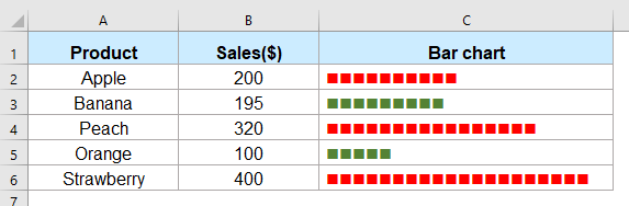
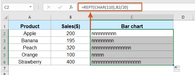
With this REPT function, you can also create a simple in-cell bar chart based on the cell value as below screenshot shown.
1. In a blank cell where you want to insert the bar chart, enter the following formula:
Note: In the above formula, char(110) is the character that you want to repeat which will display the character with an ASCII code 110; B2/20 calculates the number of times that you want to repeat based on, you can change the calculation based on your data.
2. Then, drag the fill handle down to the cells you want to apply this formula, and you will get the following result:
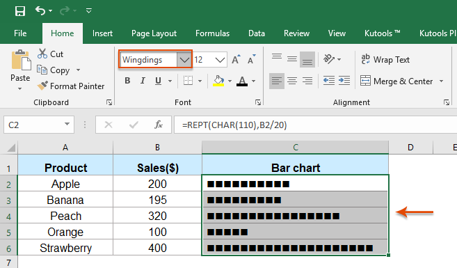
3. Then, select the formula cells, and change the text font to Wingdings formatting, some solid squares will be displayed, if you change the number in Column B, the bar chart will be changed as well, see screenshot:
Tips: If you want to show specific color based on the number, for example, to format the bar chart red color when data is greater than or equal to 200, if the data is less than 200, format it as green.
1. Select the cells with the bar chart, and then click Home > Conditional Formatting > New Rule.
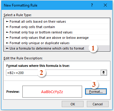
2. In the New Formatting Rule dialog box:
- (1.) Select Use a formula to determine which cells to format in the Select a Rule Type list box;
- (2.) In the Format values where this formula is true text box, enter this formula: =B2>=200.
- (3.) Click Format button to choose a font color as you need.
3. Then click OK to close this dialog box, please repeat the above steps to create a new rule for the data less 200 in green color.
More Functions:
- Excel RIGHT Function
- RIGHT function is used to return the text from right of the text string.
- Excel NUMBERVALUE Function
- The NUMBERVALUE function help to return the real number from number is stored as text.
- Excel SEARCH Function
- The SEARCH function can help you to find the position of a specific character or substring from the given text string.
The Best Office Productivity Tools
Kutools for Excel - Helps You To Stand Out From Crowd
Kutools for Excel Boasts Over 300 Features, Ensuring That What You Need is Just A Click Away...
Office Tab - Enable Tabbed Reading and Editing in Microsoft Office (include Excel)
- One second to switch between dozens of open documents!
- Reduce hundreds of mouse clicks for you every day, say goodbye to mouse hand.
- Increases your productivity by 50% when viewing and editing multiple documents.
- Brings Efficient Tabs to Office (include Excel), Just Like Chrome, Edge and Firefox.